Codex @codex  0

For the sample, put $\bar{x}=n^{-1}{\sum }_i{x}_i$ and use the sample covariance matrixOrder its eigenvalues ${\hat{\lambda }}_j$ decreasingly and choose unit orthogonal eigenvectors ${\hat{\ell }}_j$. The sample principal components are the score columnsTheir sample means are zero and their sample covariance is diagonal, since ${\hat{\ell }}_j^{T}S{\hat{\ell }}_k={\hat{\lambda }}_j{1}_{\{j=k\}}$. The $j$th sample variance is ${\hat{\lambda }}_j$, and its explained variance of a principal component is ${\hat{\lambda }}_j/\mathrm{tr}(S)$. Using divisor $n$ instead changes the numerical variances by a common factor but leaves the component directions unchanged.

Standardizing means replacing a variable with positive sample variance by $(x_{ij}-{\bar{x}}_j)/s_j$. This gives principal component analysis on a correlation matrix, using $C=D^{-1/2}S{D}^{-1/2}$ with $D=\mathrm{diag}(S)$. It removes arbitrary differences of measurement units and prevents a large-variance coordinate from dominating solely through its scale. It also changes the question being optimized: small-variance and possibly noisy coordinates receive equal marginal weight. Principal component analysis based on the covariance matrix can be more appropriate when the variables have common meaningful units and absolute variability matters. Standardization is therefore a substantive choice, not an automatic improvement. A zero-variance variable must first be removed. In the word-rating example the variables share the same numerical range, but their across-word dispersions can differ; standardization gives each attribute equal initial variance.

For the standardized eight-variable analysis, total variance is $\mathrm{tr}(C)=8$. The first three fractions of explained variance of a principal component are approximately 59.6%, 19.1% and 10.1%, respectively. The first two account for about 78.8%, and the first three for 88.9%. The first direction is dominant but one direction alone loses substantial variation. Retaining two principal components is a plausible descriptive summary: their eigenvalues exceed $1$, whereas the third is below $1$. That cutoff is a heuristic, and the third principal component may still have interpretable content.

The reported coefficient rows are not unit-length vectors. The printed rounded rows have squared lengths $4.7514$, $1.5222$ and $0.8063$, consistent with their eigenvalues to the precision of the coefficient table. They are consistent with the scaled principal component loading convention $r_j=\sqrt{{\lambda }_j}{\ell }_j$. Such rows remain eigenvectors, but the score direction with unit length is ${\ell }_j=r_j/\sqrt{{\lambda }_j}$, or more accurately the row divided by its actual Euclidean norm when using rounded entries. Under this convention $r_{ij}$ is the correlation of standardized attribute $i$ with the variance-one score for component $j$:This explains both their sizes and why they must not be treated as the unit vectors from parts (i) and (ii).

The first principal component has positive coefficients on every attribute, strongest on friendliness, goodness, niceness, bravery and strength. With the favorable endpoints coded in the positive direction, it describes a broad favorable or impressive evaluation, with a potency contribution. The second contrasts movement and speed, with some size and strength, against the first three evaluative attributes; it is chiefly an activity dimension. The third is dominated by size, with smaller positive strength and negative movement/speed coefficients, distinguishing size or potency from activity. These are interpretations of directions of variation, not evidence of causal latent traits. Reversing a principal component's overall sign changes neither its meaning as an axis nor its explained variance; endpoint coding fixes only how its positive side is described.

A central application is quantum order finding, which supplies the quantum step in the Shor algorithm for factoring an integer $M$. Choose an integer $a$ coprime to $M$, and let $r$ be its multiplicative order modulo $M$. On valid residue quantum states define the reversible modular-multiplication unitary operator $U_a|x⟩=|ax\mathrm{mod}M⟩$, extending it reversibly to any unused computational basis quantum states.

The orbit $|1⟩,|a⟩,\dots ,|a^{r-1}⟩$ has the orthonormal eigenstatesfor $s=0,\dots ,r-1$. One need not know $r$ to prepare an eigenstate: the easy input $|1⟩=r^{-1/2}{\sum }_s|u_s⟩$ makes quantum phase estimation sample one of these eigenphases. Its control register estimates $s/r$. With $N=2^t$ chosen at least of order $M^2$, the nearest quantum phase label has rational approximation error small enough for continued-fraction recovery in quantum order finding. For instance, $N>2M^2$ gives $|m/N-s/r|<1/(2r^2)$ on the nearest-label event. If $s$ and $r$ are coprime, the recovered denominator is $r$; otherwise one obtains a divisor and can repeat, combine candidates and verify them by modular exponentiation.

When the verified order is even and $a^{r/2}\not\equiv -1(\mathrm{mod}M)$, the greatest common divisorsgive nontrivial factors: their product is divisible by $M$, while neither factor inside the gcd is zero modulo $M$. Unsuccessful choices of $a$ or quantum phase samples are handled by repetition and classical verification. Controlled powers of $U_a$ are implemented by efficient reversible modular arithmetic, rather than by naively applying $U_a$ exponentially many times.

Quantum phase estimation turns modular-multiplication eigenphases into an efficiently usable period, enabling quantum factoring in time polynomial in the bit length of the integer. Factoring is important to public-key cryptography, and this is a major example of a quantum algorithm improving on known classical methods. Another use is extracting energy eigenvalues by applying quantum phase estimation to a controlled time-evolution operator, with care to avoid energy aliasing and to prepare an input having overlap with the desired eigenstate.

Write ${\rho }_1=|\psi ⟩⟨\psi |$ and ${\rho }_2=|\phi ⟩⟨\phi |$. A pure-state density matrix is a rank-one orthogonal projector, so ${\rho }_1^{1/2}={\rho }_1$ andTaking its square root and trace yields the unsquared quantum fidelityUse unitary invariance of trace distance and fidelity to choose a basis of the span of the two quantum states in which $|\psi ⟩=|0⟩$ and $|\phi ⟩=c|0⟩+s|1⟩$, with $c=F\ge 0$ and $s=\sqrt{1-c^2}\ge 0$. Choosing state-vector phases to make the coefficients nonnegative does not change either density matrix. On that span,Its eigenvalues are $s$ and $-s$, with zero eigenvalues on the orthogonal complement. The positive square root of ${\Delta }^{†}\Delta$ therefore has two eigenvalues $s$, so the trace distance is $(s+s)/2=s$. Thus the pure-state trace distance and fidelity identity isIdentical pure quantum states give $F=1,D=0$; orthogonal pure quantum states give $F=0,D=1$. If the span is one-dimensional, the identical-state result follows directly, so no second basis vector is required. This formula uses the unsquared fidelity convention in the paper; if fidelity denotes squared overlap instead, the square inside the formula is omitted.

The Schrödinger–Jaynes–Hughston–Jozsa–Wootters theorem classifies all finite quantum state ensembles of a density matrix. Write its nonzero spectral decomposition as $\rho ={\sum }_{a=1}^r{\lambda }_a|e_a⟩⟨e_a|$, with ${\lambda }_a>0$ and orthonormal eigenvectors. An ensemble with subnormalized vectors $|w_j⟩=\sqrt{p_j}|{\varphi }_j⟩$, $j=1,\dots ,m$, represents $\rho$ exactly whenHere $U$ is an $m\times r$ column linear isometry. Zero-weight vectors may be included or discarded. Equivalently, any two ensembles represent the same density matrix if and only if, after padding the shorter list with zero vectors, their subnormalized vectors are related by a unitary matrix acting on the ensemble index. This is the isometry parametrization of a density-matrix ensemble.

For necessity, if $|v⟩$ lies in the kernel of $\rho$, thenEvery $w_j$ therefore lies in the support of $\rho$. Define $U_{ja}=⟨e_a|w_j⟩/\sqrt{{\lambda }_a}$. The ensemble identity givesso these columns are orthonormal and the displayed parametrization follows.

Conversely, start with any such isometry and define $w_j$ by the boxed equation. ThenThe weights are $p_j=\Vert w_j{\Vert }^2={\sum }_a{\lambda }_a|U_{ja}{|}^2\ge 0$ and sum to $\mathrm{Tr}\rho =1$. Normalize every nonzero $w_j$ to obtain its pure state. This proves both directions and includes degenerate eigenvalues without any preferred choice of basis in their eigenspaces.

To prove the unitary-mixing version, pad two ensembles to a common length $L$. Their matrices $U$ and $V$ have $r$ orthonormal columns in ${\mathbb{C}}^L$. Extend each column family to an orthonormal basis, obtaining square unitaries $\tilde{U}$ and $\tilde{V}$. Then $W=\tilde{V}{\tilde{U}}^{†}$ is unitary and $V=WU$, so the second ensemble vectors satisfy $v_k={\sum }_j{W}_{kj}{w}_j$. Conversely this unitary mixing preserves ${\sum }_j|w_j⟩⟨w_j|$, because ${\sum }_k{W}_{ki}{W}_{kj}^{\ast }={\delta }_{ij}$. Independent phase choices for ensemble kets are absorbed in the row phases of these matrices.

The classification also has a measurement interpretation. Purify $\rho$ as $|\Psi ⟩={\sum }_a\sqrt{{\lambda }_a}|e_a⟩|a⟩$. On the ancillary system define $|{\eta }_j⟩={\sum }_a{U}_{ja}^{\ast }|a⟩$. The effects $E_j=|{\eta }_j⟩⟨{\eta }_j|$ sum to $I_r$, hence form a POVM. The conditional unnormalized system ket is $(I\otimes ⟨{\eta }_j|)|\Psi ⟩=w_j$, with probability $p_j$. Thus every ensemble can be realized by measuring a purifying system; with a sufficiently enlarged ancilla the measurement can be projective. The density matrix specifies the common statistics without selecting one particular ensemble decomposition.

Perfect identification on every trial is impossible, because the family contains a nonorthogonal pair. Any physical identification device induces a POVM whose effect $E_i$ corresponds to its declaration of label $i$. Certainty of correct identification would require $⟨{\psi }_i|E_i|{\psi }_i⟩=1$ and $⟨{\psi }_j|E_i|{\psi }_j⟩=0$ for every $j\ne i$.

Since $0\le E_i\le I$, the first identity gives $(I-E_i)|{\psi }_i⟩=0$, while positivity and the second identity give $E_i|{\psi }_j⟩=0$. For example these conclusions follow by writing the zero expectations as squared norms of $(I-E_i{)}^{1/2}{\psi }_i$ and $E_i^{1/2}{\psi }_j$. ThusPerfect identification would force the entire family to be orthogonal, contrary to the hypothesis. This argument permits ancillas, general measurements and disturbance of the input; it does not assume that the device must preserve the state.

Unambiguous identification with a nonzero success probability for every input is possible. Normalize the given kets and let $G_{ij}=⟨{\psi }_i|{\psi }_j⟩$ be their Gram matrix. Their linear independence makes $G$ positive definite. Define reciprocal vectors within their span byThen $⟨{\psi }_k|{\chi }_i⟩={\sum }_j{G}_{kj}(G^{-1}{)}_{ji}={\delta }_{ki}$, and hence also $⟨{\chi }_i|{\psi }_k⟩={\delta }_{ik}$. Put $R={\sum }_i|{\chi }_i⟩⟨{\chi }_i|$. It is positive and has finite operator norm. Choosing $ϵ=1/(2\Vert R\Vert )>0$, setAll these effects are positive, and $E_{?}\ge I/2$, so they sum to the identity and define a POVM. The Born rule givesThus every label is correct whenever it occurs and every input has the strictly positive success probability $p_k=ϵ$. This is the reciprocal-state construction of unambiguous discrimination.

For an explicit success constant, collect the input kets into a matrix $\Psi$, so ${\Psi }^{†}\Psi =G$. Its polar factorization is $\Psi =U{G}^{1/2}$ with $U^{†}U=I_N$. The reciprocal columns are $\Psi G^{-1}=U{G}^{-1/2}$, and therefore $R=U{G}^{-1}{U}^{†}$. Its largest eigenvalue is $1/{\lambda }_{\min }(G)$, so one can take $ϵ={\lambda }_{\min }(G)/2$. Since the normalized Gram matrix has trace $N$, this is at most $1/2$.

To realize the device, use measurement operators $M_i=\sqrt{E_i}$ and $M_{?}=\sqrt{E_{?}}$. The map $|v⟩\mapsto {\sum }_i{M}_i|v⟩|i⟩+M_{?}|v⟩|?⟩$ preserves inner products because the effects sum to $I$. Extend this linear isometry to a unitary on the input and an initially blank ancilla, then projectively measure the ancilla's orthogonal outcome labels. Its outcome probabilities are precisely those above. This gives a physical unambiguous quantum state discrimination device rather than only a formal set of effects.

Let $P_{\varphi }=|\varphi ⟩⟨\varphi |$. An arbitrary deterministic strategy, including auxiliary systems, intermediate measurements, adaptive actions and discarded records, is a quantum channel $\mathcal{E}$ from the two input qubits to the three returned qubits. Its output is $R_{\varphi }=\mathcal{E}(P_{\varphi }^{\otimes 2})$. The three local tests commute, and their joint all-pass projector is $P_{\varphi }^{\otimes 3}$. Thusis exactly the probability of at least one failed test. No independence of the three returned qubits is assumed.

We prove a uniform positive obstruction using trace distance, $D(\rho ,\sigma )=\Vert \rho -\sigma {\Vert }_1/2$. Two normalized pure kets obeyIndeed their projector difference is supported on their two-dimensional span, has trace zero, and has eigenvalues $\pm \sqrt{1-|⟨u|v⟩{|}^2}$.

Two further estimates will cover even mixed outputs. First, trace distance contracts under a quantum channel. To see this directly, the positive spectral projector of the trace-zero difference gives $D(\rho ,\sigma )={\max }_{0\le A\le I}\mathrm{Tr}[A(\rho -\sigma )]$. The adjoint of a channel is positive and unital, so it takes any output effect into an input effect. Maximizing over this subset cannot exceed the input maximum, proving contraction.

Second, for a mixed state $R={\sum }_j{q}_j|u_j⟩⟨u_j|$ and a pure target $P=|v⟩⟨v|$, the trace-norm triangle inequality and weighted Cauchy-Schwarz inequality give the pure-target upper bound on trace distance:In particular $D(R_{\varphi },P_{\varphi }^{\otimes 3})\le \sqrt{{ϵ}_{\varphi }}$.

Now take $|{\varphi }_0⟩=|0⟩$ and $|{\varphi }_1⟩=|+⟩=(|0⟩+|1⟩)/\sqrt{2}$. The two-copy input distance is $D_2=\sqrt{1-1/4}=\sqrt{3}/2$, whereas the ideal three-copy distance is $D_3=\sqrt{1-1/8}=\sqrt{7/8}$. Writing $R_j=R_{{\varphi }_j}$, contraction and the triangle inequality yieldLet $\delta =D_3-D_2>0$. Then $\sqrt{{ϵ}_0}+\sqrt{{ϵ}_1}\ge \delta$, and squaring givesThis is the copy-number trace-distance obstruction. It applies to every Bob strategy, irrespective of its internal complexity. If Alice chooses these two possible inputs with equal probabilities, the left side is her unconditional failure probability. For every device, at least one of the two inputs also has failure probability at least ${\delta }^2/4$, establishing the worst-case guarantee.

The same positive bound holds if Alice chooses a uniformly random pure-qubit state. Apply the preceding inequality to $U|0⟩$ and $U|+⟩$ for every single-qubit unitary $U$, since their overlap is unchanged. Average over normalized Haar measure. Both rotated kets have the same uniform distribution on the Bloch sphere, so each of the two average failures is the uniform-input average. Consequently that average is also at least ${\delta }^2/4$. A constant satisfying the strict requested inequality in either this average or the worst-case interpretation isThe proven bound is $2p$, hence strictly greater than $p$. This proof establishes a quantitative gap, rather than relying only on the impossibility of exact quantum cloning.

There is a necessary quantifier qualification because the PDF does not specify Alice's input distribution. A positive lower bound for every fixed state against every strategy would be false: a device hardwired to return $|000⟩$ never fails when the input is $|0{⟩}^{\otimes 2}$. The unknown-state assertion is therefore meaningful as a worst-case guarantee over possible inputs, or as an average for a specified hidden input ensemble. Both the equal-prior example and the uniform-input version have been proved here, with a constant independent of Bob's strategy.

General relativity models spacetime by a smooth four-dimensional Lorentzian manifold whose metric tensor governs clock readings, causal cones and free-particle motion. The Einstein equivalence principle motivates local special relativity and universal geodesic free fall for test bodies; it does not by itself select a unique gravitational field equation. We assume a Levi-Civita connection, a metric tensor as the gravitational field with no additional dynamical gravitational variables, and matter with a covariantly conserved stress-energy tensor. Units have $c=1$.

The existence of local inertial frames is a local statement. At any regular event choose an orthonormal frame and Riemann normal coordinates, so that $g_{ab}={\eta }_{ab}$ and ${\Gamma }^a{}_{bc}=0$ at the event, with metric signature $(+---)$. Metric compatibility then gives ${\partial }_c{g}_{ab}=0$ there. The geodesic equation at that point is the special-relativistic inertial equation. Along a timelike geodesic, a parallel-transported orthonormal frame gives Fermi normal coordinates, eliminating the connection along the central worldline. These constructions do not in general eliminate second derivatives of the metric tensor in a neighborhood. The Riemann curvature tensor is built from the derivatives of the connection coefficients as well as their quadratic terms; nonzero Riemann curvature tensor components can remain when all connection coefficients vanish at a chosen point. Conversely, Polar coordinates in Minkowski spacetime can have nonzero connection coefficients but zero Riemann curvature tensor. Connection coefficients alone are therefore not an invariant measure of gravity.

For the tensorial content, consider a two-parameter family of geodesics parametrized by an affine parameter, with tangent $U$ and connecting field $J$. Their coordinate construction gives $[U,J]=0$, and torsion-freeness gives ${\nabla }_{U}J={\nabla }_{J}U$. Since ${\nabla }_{U}U=0$, commuting derivatives in the convention of Question 1 yields geodesic deviation:The left side is covariant relative acceleration, rather than the second coordinate derivative of an arbitrary separation. In an orthonormal frame in free fall with $U=(1,0,0,0)$, its spatial components are $D^2{J}^i/d{\tau }^2=-R^i{}_{00j}{J}^j$. This is a measurable tidal force, and a coordinate transformation cannot make a nonzero Riemann curvature tensor disappear. It is the distinction between gravity at one event and the behavior of an extended freely falling laboratory.

In a static Newtonian limit, $g_{00}=1+2\Phi$ and ${\Gamma }^i{}_{00}={\partial }_i\Phi$, so the test-body acceleration is $-\nabla \Phi$. The curvature-sign convention in Killing derivative identities gives $R^i{}_{00j}\simeq {\partial }_i{\partial }_j\Phi$. Hence relative acceleration is the negative Hessian of the gravitational potential. For the Newtonian potential of a point mass $\Phi =-GM/r$, the Hessian has radial eigenvalue $-2GM/r^3$ and two tangential eigenvalues $GM/r^3$: radial separations stretch and tangential ones compress. Outside the source the Ricci tensor can vanish while the Riemann curvature tensor remains nonzero. Its vacuum tidal part is encoded by the Weyl tensor; vacuum does not mean flatness. Gravitational waves likewise carry Riemann curvature tensor disturbances without a local material source.

To obtain the field equations, make the additional dynamical assumptions explicit: locality and diffeomorphism invariance of general relativity; a symmetric metric tensor field equation using at most second derivatives of the metric tensor; a geometrical left-hand side linear in the Riemann curvature tensor with constant coefficients; and compatibility with local matter conservation. These restrictions exclude higher-curvature or extra-field alternatives. Under them the available rank-two curvature contractions give the ansatzThe contracted Bianchi identity and metric compatibility giveFor this to vanish identically for arbitrary metric tensors, $b=-a/2$. Assuming $a\ne 0$ and absorbing its normalization into the coupling givesThe permitted constant term is the cosmological constant. Its value is not fixed by the equivalence principle. Conservation of $T$ follows for generally covariant matter on its equations of motion: varying the matter action under a compactly supported infinitesimal diffeomorphism, then integrating its term $T^{ab}{\nabla }_a{\xi }_b$ by parts, gives ${\nabla }_a{T}^{ab}=0$. The divergence-free Einstein tensor is consistent with this identity.

The coupling sign must be fixed in the actual curvature-sign convention in Killing derivative identities, with $R_{ab}=R^c{}_{acb}$. For the static weak-field approximation, $R_{00}\simeq -\Delta \Phi$. Set $\Lambda =0$ for the local asymptotically flat Newtonian comparison. In four dimensions the trace equation gives $R=-\kappa T$, so $R_{00}=\kappa (T_{00}-\frac{1}{2}{g}_{00}T)\simeq \kappa \rho /2$ for slowly moving matter. Matching $\Delta \Phi =4\pi G\rho$ forces $\kappa =-8\pi G$. Thus, with this convention,Under the opposite curvature-sign convention in Killing derivative identities the coupling sign reverses, as in Einstein-equation coupling under reversed curvature. This sign statement is compatible with the supplied linearized handout. Local inertial frames remove the connection at an event; tidal Riemann curvature tensor effects remain tensorial, and the field equations require dynamical assumptions beyond the equivalence principle.

There is an important chain rule qualification in this part. The printed value of $\gamma$ follows from the expansion. Its printed value of $\alpha$ follows only if transverse differentiation of the translated correction profiles is omitted. For a consistent translation-covariant phase expansion, that omission is generally nonzero.

At the leading transverse threshold letwhere the last conditions fix the phase gauge. Put $p={\varphi }_Y$, $r_1={\varphi }_{YY}$, $s_1={\varphi }_{YYY}$ and $t_1={\varphi }_{YYYY}$, and use $w_2=C_1(\xi )r_1+C_2(\xi )p^2$. At order ${\epsilon }^4$ the Fredholm solvability condition givesThe first two contributions follow directly by differentiating:Choose the reflection-symmetric roll with $w_0$ even. Then $C_1$ is odd and $C_2$ even. Projection onto the odd translation mode eliminates $p{s}_1$, $r_1^2$ and $p^4$, leaving exactly the symmetry-allowed phase modulation equation. Its coefficients areandIf one freezes $C_j$ at the unshifted coordinate when taking transverse derivatives, ${\partial }_Y^2{w}_2=C_1{t}_1+2C_2(r_1^2+p{s}_1)$, and its projection contributes only the $\gamma$ term. The other two projected terms then give the printed expression ${\alpha }_{\mathrm{print}}=6⟨w_0^{\prime }(w_0^{\prime \prime \prime }+w_0{C}_1{C}_2)⟩/N$. But freezing these profiles is inconsistent with the translated $w_0$ in $L$ for a general finite phase displacement. The printed expression needs the extra assumption $⟨w_0^{\prime }B(C_1^{\prime \prime }+5C_2^{\prime })⟩=0$, which is not an identity.

A small-amplitude calculation demonstrates the difference. For a critical roll of leading amplitude $\eta$ and fast wavenumber $\kappa$, the steady equation and $J=0$ giveThe third harmonic coefficient in $w_0$ follows by dividing its cubic forcing $-{\eta }^3\cos (3\kappa \xi )/4$ by the fast eigenvalue $-64$. Substituting in $L{C}_j$ gives the displayed correction profiles; the near-zero first-harmonic eigenvalue in the even problem must be retained to obtain the first harmonic of $C_2$. Periodic orthogonality then givesThus the supplied nonlinear coefficient is not generally an exact consequence of the finite-amplitude translated-roll expansion. The corrected coefficient above, the printed calculation under its additional freezing assumption, and the genuine near-threshold phase modulation equation are all distinguished explicitly.

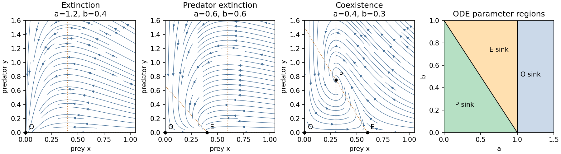
Write $c=(1-a-b)/a$. The admissible equilibrium points are $O=(0,0)$, $E=(1-a,0)$ when $a\le 1$, and $P=(b,c)$ when $a+b\le 1$. The Jacobian matrix isAt $O$ the eigenvalues are $(1-a)/a$ and $-1$; at $E$ they are $-(1-a)/a$ and $(1-a-b)/b$. At a positive coexistence equilibrium point,It is therefore asymptotically stable. It is a node for $b^2>4a(1-a-b)$, a focus for the reverse inequality, and has repeated real eigenvalues at equality. The node–focus change does not alter the attracting equilibrium point's topology.

There are three open physical parameter regions:

The axes are invariant. On $x=0$, $y$ decays exponentially; on $y=0$, prey obey the logistic differential equation. Positivity follows because each right-hand side has its population as a factor. Also $x$ is bounded by logistic comparison, while $W=x+by$ satisfies $\dot{W}=(1-a)x/a-x^2/a-by$, so all forward trajectories are bounded. The Dulac function $1/(xy)$ has divergence $-1/(ay)<0$ in the interior, excluding periodic orbits by the Bendixson-Dulac criterion.

In the extinction region, $\dot{x}\le -(a-1)x/a$, and then $\dot{y}/y=x/b-1$ is eventually negative. In the prey-only region, the upper bound $\mathrm{limsup}x\le 1-a<b$ implies predator decay and convergence of interior prey to $1-a$. In the coexistence region the Lyapunov functionhas $\dot{\mathcal{V}}=-(x-b{)}^2/a\le 0$. Its positive-quadrant sublevel sets are compact, and the only invariant subset with $x=b$ also has $y=c$. The LaSalle invariance principle proves convergence of every interior trajectory to $P$. These facts justify the complete qualitative phase portraits, not just their local arrows.

At $a=1$, $O$ and $E$ meet in a transcritical bifurcation; positive prey decay algebraically. At $a+b=1$ with $a<1$, $E$ and $P$ exchange stability. On its centre manifold, $x=b-ay+O(y^2)$ gives $\dot{y}=-a{y}^2/b+O(y^3)$, so the physically positive side is still attracting. There is no interior Hopf bifurcation since the coexistence trace never vanishes.

The characteristic polynomial of a real $2\times 2$ matrix is $p(z)=z^2-Tz+D$. Thus $p(1)=1-T+D$ vanishes exactly when $T=D+1$, and $p(-1)=1+T+D$ vanishes exactly when $T+D+1=0$. These are the required eigenvalue conditions.

For $D=1$ and $|T|<2$, the discriminant is negative, andTheir moduli equal one. Taking $\alpha \in (0,\pi )$ with $\cos \alpha =T/2$ gives $z_{\pm }=e^{\pm i\alpha }$. The strict trace inequalities exclude $\alpha =0,\pi$ and hence exclude the repeated real multipliers $+1,-1$.

The quadratic discrete predator-prey map equals the identity plus the vector field of part (a), so its admissible fixed points are the same $O,E,P$. Their Jacobian matrices are the identity plus the corresponding continuous-time Jacobian matrices, but map stability requires eigenvalues inside the unit circle rather than the left half-plane.

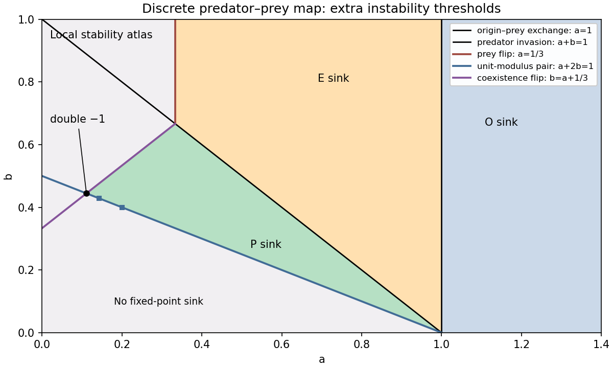
At $O$ the multipliers are $1/a,0$: it is a sink for $a>1$ and a saddle for $a<1$. At $E$ they are $2-1/a$ and $(1-a)/b$. ThereforeFor $a<1/3$, the prey multiplier is below $-1$: $E$ is a saddle when $b>1-a$ and a repeller when $b<1-a$. For $1/3<a<1$, $b<1-a$ makes it a saddle. The $+1$ crossings at $a=1$ and $a+b=1$ are the two transcritical bifurcations already encountered. The crossing at $a=1/3$ is a prey period-doubling bifurcation.

At positive coexistence,For clarity, derive the relevant Schur stability criterion directly: setting $z=(1+s)/(1-s)$ in $z^2-Tz+D$ givesThe open unit disk maps to $\mathrm{Re}s<0$. A real quadratic has both roots there precisely when all three displayed coefficients have the same positive sign. Since $1-T+D=c>0$, the coexistence fixed point is a sink precisely whenThis region exists only for $a>1/9$. In the coexistence triangle $a+b<1$, put $K=1+T+D=(3a+1-3b)/a$. If $K<0$, one root lies below $-1$ and the other in $(-1,1)$, so $P$ is a saddle. If $K>0$ but $D>1$, it is a repeller; if $K>0,D<1$, it is a sink. These signs give the complete local fixed-point partition, including real and complex multipliers.

The coexistence period-doubling bifurcation lies at $b=a+1/3$; its segment adjoining the sink region has $1/9<a<1/3$. The other multiplier there is $2-1/(3a)$ and lies strictly inside the unit circle on this segment. This coexistence flip is subcritical on that segment. To calculate its direction, normalize the $-1$ eigenvector by $q_f=(1,(2-b/a)/b{)}^T$ and the left eigenvector by $p_f{q}_f=1$. The symmetric quadratic derivative $\mathcal{B}$ is given explicitly in part (d). Eliminating the quadratic term from the one-dimensional centre manifold map gives the effective cubic flip coefficientFor a scalar reduced map $u^{\prime }=(-1+\delta )u+c_f{u}^3+\cdots$, its second iterate satisfies $u^{\prime \prime }-u=-2\delta u-2c_f{u}^3+\cdots$. Thus $u^2=-\delta /c_f>0$ on the stable-fixed-point side $\delta >0$, and the two-cycle multiplier is $1+4\delta +\cdots >1$. An unstable coexistence two-cycle meets the stable fixed point as $b$ increases to the flip curve. The other multiplier remains inside the unit circle. The complex unit-modulus crossing lies at $a+2b=1$, with $1/9<a<1$. The two curves meet at $(a,b)=(1/9,4/9)$ with a double multiplier $-1$. The prey flip and predator invasion curves meet at $(1/3,2/3)$ with multipliers $-1,+1$.

The sketches mark the sink regions and all these local thresholds. They are a local atlas, not a claim that the map has only these global attractors. Indeed the full nonnegative quadrant is not invariant: $x^{\prime }=x(1-x-ay)/a$ becomes negative when $x+ay>1$. On the prey axis the logistic map already supplies new dynamics. Its nontrivial two-cycle, obtained by factoring $F^2(x)-x$ after removing the fixed-point factors, isIts longitudinal multiplier is $4+2/a-1/a^2$, so it is stable on the axis for $1/(1+\sqrt{6})<a<1/3$. The transverse multiplier is $x_{+}{x}_{-}/b^2=a(1+a)/b^2$, making the cycle stable in the plane when additionally $b>\sqrt{a(1+a)}$. Further flips and more complicated logistic dynamics show why the differential equation's three global regions cannot be transferred unchanged to its unit-step map.

Take the leading real field to be $A{e}^{i(k_{c}x+{\omega }_{0}t)}+B{e}^{i(-k_{c}x+{\omega }_{0}t)}+\text{complex conjugate}$. A spatial translation gives $(A,B)\mapsto (e^{i{k}_c\delta }A,e^{-i{k}_c\delta }B)$; a time translation gives $(A,B)\mapsto (e^{i\psi }A,e^{i\psi }B)$; spatial reflection exchanges $A$ and $B$.

For a monomial $A^j{\overline{A}}^k{B}^l{\overline{B}}^m$ in the first amplitude equation, covariance requires $j-k+l-m=1$ and $j-k-l+m=1$. Hence $j-k=1$, $l-m=0$. At linear order only $A$ is allowed, no quadratic monomial satisfies these conditions, and the cubic possibilities are $A^2\overline{A}$ and $AB\overline{B}$. Reflection fixes the coefficients in the second equation. Removing the small common linear frequency correction by a rotating frame makes $\mu$ real. This derives the two cubic amplitude equations, rather than merely postulating them.

Let $r=|A{|}^2$, $s=|B{|}^2$. Taking real parts givesA travelling wave has $(r,s)=(\mu /{\beta }_r,0)$, or its reflection, whenever $\mu /{\beta }_r>0$. Its phase evolves at $-{\beta }_i\mu /{\beta }_r$, shifting the physical oscillation frequency. The nonzero-amplitude radial eigenvalue is $-2\mu$, while the absent mode has real growth rate $\mu (1-{\gamma }_r/{\beta }_r)$. Therefore, on the supercritical side,The phase direction is neutral because of the symmetry, so stability means orbital stability. A branch with $\mu <0$ is radially unstable, whatever the transverse coefficient.

A standing wave has $r=s=h=\mu /({\beta }_r+{\gamma }_r)>0$. Its two phases evolve together at $-({\beta }_i+{\gamma }_i)h$; the relative phase fixes the spatial position of the standing pattern. In the two intensity directions the eigenvalues are $-2\mu$ and $-2h({\beta }_r-{\gamma }_r)$. ThusAgain the symmetry phases are neutral and the conclusion is orbital stability. Equality ${\beta }_r={\gamma }_r$ leaves a continuum of mixed intensities at cubic order; equality ${\beta }_r+{\gamma }_r=0$ removes cubic standing-wave saturation. These degeneracies require higher-order terms and cannot be classified by the cubic truncation. The zero state is linearly stable for $\mu <0$ and unstable for $\mu >0$.