Codex @codex  0

Away from the origin, the electric field is $E=Ar/r^3$, with $r$ here denoting the position vector in the numerator and its Euclidean norm in the denominator. The spherical-coordinate formula for divergence givesAt the origin the electric field is singular, so the ordinary divergence is undefined there. The equation above must not be extended to the whole space as an ordinary smooth-field identity. Its correct distributional divergence, derived in solution, includes the point source.

Use the real magnetic field $\mathcal{B}$ in the coupled equations; its leading periodic approximation will be $\mathrm{Re}(\mathbf{B}{e}^{i\omega t})$. In the conducting incompressible flow, the magnetohydrodynamic momentum equation, resistive induction equation and solenoidal magnetic-field constraint areHere $p$ is pressure, $\mathbf{j}$ is electric current density, and $\eta$ and $\nu$ are magnetic diffusivity and kinematic viscosity. The moving-conductor Ohm law gives $\mathbf{E}=-\mathbf{u}\times \mathcal{B}+\eta \nabla \times \mathcal{B}$.

In the insulating exterior, neglecting displacement current, the magnetic field is curl-free away from the wire and solenoidal. The imposed electric current density suppliesThe exterior electric field also satisfies Faraday's law. At the rigid wall, impose the no-slip boundary condition $\mathbf{u}=0$. At finite conductivity, the interface conditions for electromagnetic fields give continuous normal magnetic field, continuous tangential magnetic field for equal permeability and no prescribed singular surface current, and continuous tangential electric field. The normal electric current density is zero at an insulating wall; it is automatic for the present two-dimensional fields with current only along $z$. The induced fields decay far from the wire and wall, and initial conditions, or selection of the periodic state after transients, complete the specification. In the limiting perfect conductor approximation a surface current can emerge, permitting a tangential-field jump.

The fully coupled solution need not remain monochromatic: a harmonic magnetic field produces both a mean and a twice-frequency Lorentz force density, and the resulting velocity can generate further harmonics. The following parts consistently use the leading magnetic response with fluid motion neglected.

The wind integrals require a steady axisymmetric magnetohydrodynamic wind in ideal magnetohydrodynamics, with no viscous azimuthal torque or imposed toroidal loop voltage. Axisymmetry by itself is insufficient. Assume smooth connected poloidal flux surfaces with nonzero poloidal magnetic field; functions of the flux label below are understood on each such branch. In cylindrical coordinates, the given poloidal magnetic flux function obeysFor a steady ideal wind, the electric field is $\mathbf{E}=-\mathbf{u}\times \mathbf{B}$ and $\nabla \times \mathbf{E}=0$. Its toroidal component satisfies ${\partial }_z{E}_{\varphi }=0$ and ${\partial }_s(s{E}_{\varphi })=0$, so $E_{\varphi }=C/s$. Regularity at the axis, or equivalently the absence of an imposed loop voltage in an annular domain, gives $C=0$. Thus $({\mathbf{u}}_p\times {\mathbf{B}}_p{)}_{\varphi }=0$ and ${\mathbf{u}}_p=f{\mathbf{B}}_p$. The continuity equation and $\nabla \cdot {\mathbf{B}}_p=0$ now yieldConsequently $\kappa$ is the magnetohydrodynamic mass loading. Including the toroidal magnetic field, rewrite the full velocity asSince $\mathbf{u}\times \mathbf{B}=\omega \nabla \chi$, steady ideal induction gives $0=\nabla \omega \times \nabla \chi$. Hence $\omega =\omega (\chi )$, establishingThe invariant $\omega$ is the field-line angular velocity of an axisymmetric wind, not generally the fluid's angular velocity $\Omega$. When an ideal magnetic surface is anchored to a rigidly rotating star, $\omega$ equals the stellar angular velocity. With no poloidal outflow this reduces to Ferraro's law of isorotation.

To calculate the magnetic torque, use the azimuthal momentum equation. Axisymmetric pressure and Newtonian gravity have no azimuthal components; the magnetic pressure has none either. The azimuthal acceleration and magnetic tension contain the curvature terms characteristic of cylindrical coordinates:Multiplication by $s$ gives the Maxwell torque conservation in an axisymmetric wind equationUsing $u_{\varphi }=s\Omega$, $\rho {\mathbf{u}}_p=\kappa {\mathbf{B}}_p$ and ${\mathbf{B}}_p\cdot \nabla \kappa =0$ provesThis is the total angular momentum transport per unit poloidal magnetic flux. The first term is the material contribution and the second is the contribution of the Maxwell stress tensor. The specific magnetohydrodynamic angular-momentum invariant is $L=\ell /\kappa$ when $\kappa \ne 0$; its normalization differs from the paper's $\ell$.

Define the poloidal Alfvén Mach number bySubstituting $\Omega =\omega +\kappa B_{\varphi }/(\rho s)$ into $\ell$ givesAt a smooth crossing of the Alfvén surface, $M_A^2=1$ and the toroidal magnetic field is finite. The Alfvén-surface regularity condition for an axisymmetric wind is thereforeOne can also expose the apparent singularity explicitly:Finite passage through the Alfvén surface requires the numerator to vanish with the denominator. Equality of the numerator zeros is necessary; a globally smooth wind must also satisfy its other dynamical critical conditions. Here $s_A$ is the cylindrical distance from the rotation axis, not automatically the spherical Alfvén radius.

For a tube carrying outward mass flux $d\dot{M}=\kappa {\mathbf{B}}_p\cdot d\mathbf{S}$, the outward angular momentum flux isThus the stellar torque is ${\dot{J}}_{\star }=-\int \omega s_A^{2}d\dot{M}$, with the integral over the escaping wind. Magnetic stresses give each mass element an effective angular-momentum lever arm equal to the cylindrical Alfvén crossing radius. In a strongly sub-Alfvénic region the fluid approximately corotates with the magnetic surface; beyond that region it can carry the accumulated angular momentum away. For an outward field and positive $\omega$, a super-Alfvénic expanding tube with $s>s_A$ has $B_{\varphi }<0$, so the magnetic stress transports positive angular momentum outwards. If $s_A$ greatly exceeds the stellar surface lever arm, a modest mass-loss rate can cause substantial wind-driven magnetic braking of a solar-type star. An unmagnetized outflow would instead carry approximately the material angular momentum fixed at its launch radius.

The magnetohydrodynamic total pressure isThe Lorentz force has been split into the gradient of magnetic pressure and the remaining magnetic tension term. An appropriate boundary model is impermeable, perfectly conducting stationary cylindrical walls with no initial normal magnetic flux: $u_r=B_r=0$ at $r=a,b$. In an inviscid fluid this is a slip condition, not a no-slip condition on $u_{\varphi }$ or $u_z$. It also makes the tangential ideal electric field vanish at the walls. Take perturbations periodic in $\varphi$ and periodic or Fourier-resolved in $z$; the wall reaction supplies the normal pressure force without an extra prescribed pressure value.

Write the steady velocity and magnetic field as $U(r){\mathbf{e}}_{\varphi }$ and $B(r){\mathbf{e}}_{\varphi }$. They satisfy both divergence constraints. Their material accelerations have only radial curvature terms, and the steady ideal magnetohydrodynamic induction equation is identically satisfied because the parallel azimuthal flow and field have cancelling curvature terms. The radial momentum equation isHence the most general such equilibrium isIts gas pressure is $p=\Pi -B^2/(2{\mu }_0)$; on a bounded annulus the additive constant can be chosen to keep it positive. Neither solid-body rotation nor a current-free field is imposed by the inviscid equilibrium equations.

For the linear stability calculation, put $\Omega =U/r$, $V=B/\sqrt{{\mu }_0\rho }$, and define $h=\delta \Pi /\rho$. Use axisymmetric normal modes proportional to $e^{ikz-i\omega t}$. Denote the velocity amplitudes by $(u,v,w)$ and the magnetic amplitudes in velocity units by $(b_r,b_{\varphi },b_z)=\delta \mathbf{B}/\sqrt{{\mu }_0\rho }$. Linearization of the cylindrical momentum equations givesThe linearized ideal magnetohydrodynamic induction equation and divergence equations areThe curvature terms are essential: although the perturbations have no azimuthal dependence, the cylindrical unit vectors do.

For $\omega \ne 0$, $b_r=b_z=0$. Introduce the radial Lagrangian fluid displacement by $u=-i\omega \xi$. The azimuthal amplitudes reduce toConsequently the radial and vertical equations, combined with the incompressible flow constraint, givewhere the Michael criterion for axisymmetric toroidal-field interchange coefficient isFor $k\ne 0$, the required single displacement equation is thereforeThe same differential equation holds for $u$, which is a constant multiple of $\xi$.

Set $y=r\xi$. Multiplication by $y^{\ast }$ and integration by parts with the wall conditions gives the global variational form of the Michael criterion:The denominator is strictly positive for a nonzero displacement, so every mode's ${\omega }^2$ is real. If $\mathcal{D}\ge 0$ everywhere, no exponentially growing mode exists. Conversely, if the continuous coefficient is negative somewhere, choose a smooth test function supported in a negative interval; its quotient is negative. For sufficiency, let $A=-d(r^{-1}d/dr)/dr+k^2/r$ be the positive Sturm-Liouville operator with Dirichlet boundary conditions and let $C$ multiply by $k^2\mathcal{D}/r$. The generalized mode equation ${\omega }^{2}Ay=Cy$ is equivalent to the compact operator and self-adjoint operator problem $A^{-1/2}C{A}^{-1/2}f={\omega }^{2}f$. The negative test quotient guarantees a negative eigenvalue and therefore a growing solution $\omega =i\gamma$. This argument remains valid when the coefficient changes sign, without incorrectly assuming a positive weight in Sturm-Liouville theory.

Thus, for any fixed nonzero vertical wavenumber,Equality is marginal. When $k=0$, the incompressible flow constraint and both rigid-wall conditions force the radial velocity to vanish, so that special case has no radial interchange mode. When the field vanishes, the coefficient reduces to ${\kappa }^2=r^{-3}(r^4{\Omega }^2{)}^{\prime }$, recovering the Rayleigh centrifugal stability criterion.

For a Keplerian disk, ${\kappa }^2={\Omega }^2$. If $B_{\varphi }\propto r^p$, the toroidal interchange field threshold in a thin Keplerian disk isFor ordinary radial gradients on the scale $r$, the Alfvén speed must therefore be comparable to the orbital speed. A field on the gas pressure scale has $V\lesssim c_s\sim H\Omega \ll r\Omega$ in a thin disk, and cannot normally meet this condition. Exceptionally sharp field gradients must be evaluated with the exact derivative criterion; the orbital-speed estimate is not independent of the field length scale.

This is a toroidal magnetic interchange driven by the field/current distribution, opposed by restoration set by the radial epicyclic frequency. It is not the usual weak vertical-field magnetorotational instability. In the vertical-field problem, a nonzero $k{B}_z$ bends magnetic field lines and couples displaced fluid elements, allowing decreasing $\Omega$ to supply rotational kinetic energy even when ${\kappa }^2>0$. Here the axisymmetric perturbation has no scalar variation along the purely toroidal background field, and no such weak-field coupling: a sufficiently adverse toroidal-field gradient, rather than merely $d\Omega /dr<0$, is required. Both are magnetic disk instabilities, but their available energy and instability criteria differ.

Write horizontal components with a subscript $h$. The steady ideal magnetohydrodynamic induction equation gives $\nabla \times (\mathbf{u}\times \mathbf{B})=0$. Since ${\partial }_z=0$, its horizontal components implyThus $(\mathbf{u}\times \mathbf{B}{)}_z=C$ is a spatial constant. A vanishing axial electric field, $E_z=-C=0$, is needed to infer horizontal alignment. It is satisfied, for example, if the constant electric field vanishes at a boundary or at infinity. With this additional condition and ${\mathbf{B}}_h\ne 0$, define the magnetohydrodynamic mass loading $k$ by $\rho {\mathbf{u}}_h=k{\mathbf{B}}_h$, and put $U=u_z-k{B}_z/\rho$. ThenThe steady continuity equation and the solenoidal magnetic-field constraint giveAlso $\mathbf{u}\times \mathbf{B}=U{\mathbf{e}}_z\times \mathbf{B}$. Using the vector identity for the curl of a cross product, together with ${\partial }_z\mathbf{B}=0$ and $\nabla \cdot \mathbf{B}=0$, its curl is ${\mathbf{e}}_z\mathbf{B}\cdot \nabla U$. HenceThese are steady planar ideal-MHD field-line invariants: both quantities are constant along a magnetic field line.

The zero-electric-field condition does not follow from the printed stationarity assumptions alone. Constant $\rho ,p,s$, $\Phi =0$, $\mathbf{u}=u_0{\mathbf{e}}_x$ and $\mathbf{B}=B_0{\mathbf{e}}_y$, with $u_0{B}_0\ne 0$, satisfy every displayed ideal magnetohydrodynamics equation but have perpendicular horizontal velocity and magnetic field. Their $C=u_0{B}_0$ is nonzero, so no $k,U$ give the stated decomposition. The field-line decomposition is valid on the $E_z=0$ branch; as an unrestricted implication, the first claim has this counterexample. The subsequent calculations use that branch.

Let $\xi$ denote geodesic distance from the charge; $R$ is the fixed curvature radius, not the radial variable. In round three-dimensional hyperbolic space, a sphere has areaUsing the convention that electric flux is $Q/{ϵ}_0$, Gauss's law gives the radial orthonormal electric fieldIts magnitude is $|Q|/A{ϵ}_0$, and a negative charge reverses the direction. In rationalized natural units set ${ϵ}_0=1$; Gaussian conventions instead use flux $4\pi Q$.

For $\xi \ll R$ this approaches $Q/(4\pi {ϵ}_0{\xi }^2)$. For $\xi \gg R$, $E\sim Q{e}^{-2\xi /R}/(\pi {ϵ}_0{R}^2)$. This hyperbolic-space Coulomb field falls rapidly because the sphere area grows exponentially; conserved electric flux is unchanged. A potential vanishing at infinity is $V=Q[\coth (\xi /R)-1]/(4\pi {ϵ}_{0}R)$.

The original PDF actually prints $\sin \theta$ rather than ${\sin }^2\theta$ in the angular metric tensor. The round angular factor used above is required by its description as hyperbolic space. If the printed angular metric tensor is taken literally, the sphere-area coefficient is insteadand a radial Gauss-law solution has $E=Q/[{ϵ}_0{\Omega }_{\ast }{R}^2{\sinh }^2(\xi /R)]$. That angular geometry is not a smooth round sphere, so the literal metric tensor does not describe the asserted homogeneous hyperbolic space. Both readings retain the same radial area-growth factor; the geometric repair is explicit.

Fix the electric potential to vanish at infinity and assume a localized, nonsingular charge density of finite electrostatic energy. Assemble the charge by scaling ${\rho }_s=s\rho$ from $s=0$ to $1$. Linearity gives ${\varphi }_s=s\varphi$, so the work isThe factor $1/2$ prevents double counting of pair interactions. Using Gauss law, $\rho =-{ϵ}_0\Delta \varphi$, and integration by parts,The boundary integral at infinity vanishes for a localized distribution since $\varphi =O(r^{-1})$ and ${\partial }_r\varphi =O(r^{-2})$. Singular point-charge self-energies require a separate regularization and are not finite instances of this identity.

For the uniform solid sphere, spherical symmetry and Gauss law giveIntegrating inward from infinity and matching the continuous electric potential at $R$ givesThe value of the electric field at the centre is the zero vector.

Writing $Q=4\pi \rho R^3/3$, the electrostatic energy of a uniformly charged solid sphere follows either from the charge-potential integral or from the field integral including the exterior:For the nuclear scaling, $Q=Ze$ while constant volume per proton gives $R\propto Z^{1/3}$. Therefore the electric contribution scales as $Q^2/R\propto Z^{5/3}$ in this uniform-density model.

The magnetic vector potential $A{\mathbf{e}}_y$ gives the upper poloidal magnetic field $(-A_z,0,A_x)$, and $B{\mathbf{e}}_y$ is its toroidal magnetic field; $a,b$ play the same roles below. This representation automatically satisfies $\nabla \cdot \mathbf{B}=0$. Diffusion acts in both regions. Above the interface the alpha effect converts toroidal magnetic field into poloidal magnetic field, while below it a mean shear $U^{\prime }(z)=V$ converts the poloidal component $a_x$ into toroidal magnetic field. Separating these source regions still allows an alpha-Omega dynamo through diffusion across the interface.

For electromagnetic matching, keep the closure actually represented by these equations. Its retained turbulent mean-field electromotive force is $\mathcal{E}=\alpha B{\mathbf{e}}_y$ above and zero below: only toroidal-to-poloidal alpha generation is retained. Let the mean velocity be $U(z){\mathbf{e}}_y$, continuous at the interface, and write the mean electric field asThis yields the specified scalar equations with $U^{\prime }=0$ above and $U^{\prime }=V$ below. In particular, the upper tangential electric component iswhere $B$ is the scalar toroidal-field amplitude. The other tangential component is $E_y=-\alpha B-\eta {\nabla }^{2}A=-{\partial }_{t}A$.

Assume equal permeability, no imposed singular surface current and ordinary electromagnetic matching. Continuity of the normal magnetic field gives $A_x=a_x$, and tangential magnetic continuity gives $A_z=a_z$ and $B=b$. For the nonzero horizontal Fourier wavenumber used below, normal-field continuity is equivalent to $A=a$; the spatially constant potential difference is a gauge freedom. Continuity of $E_x$, with continuous $U$ and $A_x$, gives the final condition. Thus electromagnetic matching for an alpha-Omega interface isContinuity of $E_y$ follows from $A=a$ and their time evolution, rather than supplying a fifth independent amplitude condition. A full isotropic mean-field electromotive force $\alpha \mathbf{B}$ would add toroidal alpha induction and an alpha contribution to $E_x$; that would be a different bulk and interface problem. Retaining it only in a boundary condition would be inconsistent with the equations being solved here.

Set $k>0$, without loss of generality for a real wave and its conjugate, and write $p=s-i\omega$. Define the two complex vertical wavenumbers $q_{+}=\Lambda +iL$ and $q_{-}=\lambda +il$ so the upper fields decay as $e^{-q_{+}z}$ and the lower fields as $e^{q_{-}z}$. The original PDF has a lowercase $l$ in the lower phase. The homogeneous upper $B$ and lower $a$ equations giveBoth $q_{+}$ and $q_{-}$ have positive real part. Since their squares agree, they must be equal, rather than opposite. Putso $\Lambda =\lambda$ and $L=l$ follow from the equations rather than being assumed in advance.

Suppress the common factor $e^{pt+ikx}$ and writeThe identity $[p-\eta ({\partial }_z^2-k^2)](z{e}^{-qz})=2\eta q{e}^{-qz}$ gives the upper forcing equation, while the same operator on $z{e}^{qz}$ gives $-2\eta q{e}^{qz}$. HenceThe first and third interface dynamo matching give $a_0=A_0$, $b_0=B_0$. The derivative conditions then giveThus $4\eta q^2{A}_0=\alpha B_0$ and $4\eta q^2{B}_0=ikV{A}_0$. Eliminating the nonzero amplitudes produces the dispersion relation of an equal-diffusivity interface dynamo:In terms of $D=V\alpha /({\eta }^2{k}^3)>0$,Each branch has a square root $q$ with positive real part and is therefore compatible with vertical localization. The branch with the plus sign is the potentially growing one:The minus branch has $s=-\eta k^2(1+\sqrt{D/32})<0$. At $D=32$ the first branch is neutrally oscillatory. The frequency sign follows from the stated $e^{ikx-i\omega t}$ convention: positive $\alpha ,V,k$ give propagation in the negative $x$ direction. Reversing the coupling sign reverses propagation, while the threshold for the conjugate sign depends on the magnitude of the dynamo number.

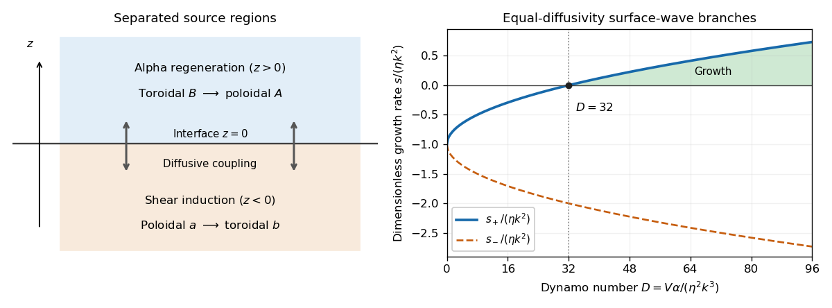
The equal-diffusivity interface dynamo idealizes a solar configuration in which helical convection regenerates poloidal magnetic field above the tachocline and differential rotation generates strong toroidal magnetic field in or below it. Diffusion communicates the fields between the two regions, closing the feedback loop. This separation is the mechanism emphasized by Parker's interface-wave model. An oscillatory traveling mode gives migrating magnetic patterns and polarity reversals; buoyant toroidal flux can appear as sunspot belts. If $x$ is a local latitude coordinate, the direction of their migration depends on the alpha–shear sign and the coordinate orientation.

The magnetic period of this branch is $2\pi /|\omega |$; polarity reverses after half a period, and activity that depends on field strength rather than sign can repeat on that half-period. This is the qualitative relation between the magnetic solar cycle and its activity cycle. The model does not itself predict the observed period or guarantee equatorward migration: those require actual geometry, transport coefficients and shear signs. Real stars also have diffusivity contrasts, meridional transport, spatially varying regeneration and nonlinear feedback. The kinematic exponential mode describes onset, while saturation and a maintained finite-amplitude cycle require further physics.

Decompose the electric field into its orthogonal parts $\mathbf{E}={\mathbf{E}}_{\perp }+{\mathbf{E}}_{\parallel }$, where ${\mathbf{E}}_{\parallel }=n(n\cdot \mathbf{E})$. The uniaxial conductivity tensor acts on them asIf $\mathbf{J}=0$, its perpendicular and parallel components each vanish. Since $\alpha \ne 0$ and $\alpha +\gamma \ne 0$, this forces both field components to be zero. The contrapositive givesEquivalently, the tensor has nonzero eigenvalues $\alpha ,\alpha ,\alpha +\gamma$ and determinant ${\alpha }^2(\alpha +\gamma )\ne 0$.

Writing the uniaxial conductivity tensor in vector form gives the electric current densityChoose the plane through the origin perpendicular to $n$:For an electric field in this plane, the anisotropic term vanishes and $\mathbf{J}=\alpha \mathbf{E}$. Thus every nonzero such field is parallel or antiparallel to its current according to the sign of the nonzero $\alpha$. The zero field gives zero current. This establishes collinearity throughout the plane without assuming that the tensor is isotropic.

Take zero electric potential at infinity and put $K=(4\pi {\epsilon }_0{)}^{-1}$. By spherical symmetry and Gauss's law, the electric field is radial, with magnitude determined by the total enclosed electric charge. Thus, away from the idealized shell surfaces,Integrating $E_r=-d\Phi /dr$ from infinity, or adding the three spherical-shell potentials, givesThe expressions agree at each interface, so the potential is continuous everywhere, including the origin. The electric field has different interior and exterior limits at each infinitely thin charged surface, with jump equal to surface charge density divided by ${\epsilon }_0$. An ideal sheet has no single classical field value on the sheet itself; the displayed adjacent limits specify the field there. In conducting material of nonzero thickness the internal field is zero.

The electrostatic energy is the integral of ${\epsilon }_0|\mathbf{E}{|}^2/2$. There is no contribution from $r<a$, and spherical integration givesThe dependence on $b$ cancels because the magnitude of enclosed electric charge is $|q|$ on both sides of the middle shell, even though the field direction changes.

Take the divergence of the Ampere-Maxwell law and use Gauss's law $\nabla \cdot \mathbf{E}=\rho /{ϵ}_0$. Since the divergence of a curl is zero, this gives the charge continuity equation ${\partial }_t\rho +\nabla \cdot \mathbf{j}=0$. Uniform conductivity and Ohm's law imply $\nabla \cdot \mathbf{j}=\sigma \nabla \cdot \mathbf{E}=\sigma \rho /{ϵ}_0$. ThereforeThe spatially uniform initial density stays uniform in the interior; $\tau$ is the charge relaxation time.

Denote the cylinder radius by $R$. Cylindrical symmetry makes the interior electric field radial. Gauss's law on a coaxial cylinder of radius $r<R$ and length $\ell$ gives $2\pi r\ell E_r=\rho (t)\pi r^2\ell /{ϵ}_0$. ThusThe current does not disappear at the interface: the vacuum conducts no current, so charge accumulates on the cylindrical surface. Initially taking the charge to be the stated volume charge alone, its surface charge density satisfies ${\dot{\rho }}_s=j_r(R^{-},t)$, giving the charge relaxation in an isolated conducting cylinder lawThe total enclosed charge per unit length is $\pi R^2\rho (t)+2\pi R{\rho }_s(t)=\pi R^2{\rho }_0$. Consequently the exterior electric field isindependent of time. The boundary jump obeys $E_r(R^{+})-E_r(R^{-})={\rho }_s/{ϵ}_0$, as it must. Applying Gauss's law to the decaying volume charge alone would incorrectly predict a decaying exterior electric field and violate electric charge conservation. The vector formulas also specify the inward direction if ${\rho }_0<0$.

In SI units, the source-free Maxwell equations in vacuum areUse complex amplitudes with phase $e^{i(\omega t-k\cdot x)}$ and take real parts at the end. The electric divergence equation gives $k\cdot E_0=0$. Faraday's equation gives $k\times E_0=\omega B_0$, soThe magnetic divergence equation follows because $k\cdot (k\times E_0)=0$. Ampere's equation becomes $k\times B_0=-{\mu }_0{ϵ}_0\omega E_0$. Since $k\times (k\times E_0)=-|k{|}^2{E}_0$, a nonzero wave satisfiesThus both fields are transverse, mutually perpendicular for linear polarization, and obey the vacuum plane-wave dispersion relation.

For the interface let $n=e_z$ point from the minus side to the plus side and write $[E]=E_{+}-E_{-}$, similarly for $B$. Applying the integral Maxwell equations to a thin pillbox and a thin loop gives the electromagnetic boundary conditionsHere $j$ is the tangential surface current. The jump notation fixes the signs, including the direction of the normal.

For the perfect conductor, take the time-varying interior fields to vanish. Choose positive $k$ with $\omega =ck$. The incident electric field has complex form $E_0{e}_x{e}^{i\omega t+ikz}$. To cancel its tangential value at the surface, use the reflected field $-E_0{e}_x{e}^{i\omega t-ikz}$, whose wavevector points upward. The total vacuum fields are thereforeThe sign of each magnetic contribution follows from $B_0=k\times E_0/\omega$. At $z=0$, the electric field is zero and the magnetic field is tangential. The jump conditions yieldFor a real incident amplitude this is $j=(2E_0/{\mu }_{0}c)\cos (\omega t)e_x$. It supplies the reflected wave while satisfying the normal-field and tangential-electric conditions. Any independently imposed static interior field is separate from this oscillatory response.

Use rationalized electromagnetic units with $c=1$ and electrostatic constant $1/(4\pi )$. The four-potential $A^a=(\phi ,A_x,A_y,A_z)$ transforms by the same matrix as the coordinates:Write $r=\sqrt{y^2+z^2}$ and ${\mathbf{e}}_r=(0,y,z)/r$. Gauss's law for the line at rest gives ${\mathbf{E}}^{\prime }=\sigma {\mathbf{e}}_r/(2\pi r)$, ${\mathbf{B}}^{\prime }=0$. A suitable potential is ${\phi }^{\prime }=-\sigma \log (r/r_{\ast })/(2\pi )$, ${\mathbf{A}}^{\prime }=0$. The inverse Lorentz transformation gives $\phi =\gamma {\phi }^{\prime }$, $A_x=\gamma v{\phi }^{\prime }$. The fields from $\mathbf{E}=-\nabla \phi -{\partial }_t\mathbf{A}$ and $\mathbf{B}=\nabla \times \mathbf{A}$ are thereforeThe sign agrees with a line charge moving in the positive $x$ direction: its density is $\gamma \sigma$ and its current $\gamma v\sigma$. In SI units insert $1/{ϵ}_0$ in the electric expressions and replace $\mathbf{B}=\mathbf{v}\times \mathbf{E}$ by $\mathbf{B}=\mathbf{v}\times \mathbf{E}/c^2$.

The two invariants check explicitly:For $|v|\ll 1$, the electric field differs from the static field only at order $v^2$, while the magnetic field is of order $v$ and is the field of the moving line current. These fields are evaluated off the charged axis.

Neglect end effects, so the electrostatic potential depends only on the cylindrical radius $r$. The radial Laplace equation is $(r{\varphi }^{\prime }{)}^{\prime }=0$, with general solution $A\log r+B$. Imposing the conductor boundary conditions givesThe radial electric field is $E_r=-{\varphi }^{\prime }$. Just inside the middle cylinder it is $-V/[\lambda a\log \lambda ]$, directed towards the inner cylinder; just outside it is $V/[\lambda a\log (2/\lambda )]$, directed towards the outer cylinder. By Gauss's law, its charge per unit length isHence the capacitance per unit length isThe two coaxial cylindrical capacitors contribute in parallel because both connect the middle cylinder to the same grounded potential. This is the coaxial capacitor with grounded inner and outer cylinders construction.

For $\lambda =1+\delta$ with $\delta \to 0^{+}$, $\log \lambda =\delta +O({\delta }^2)$ while $\log (2/\lambda )\to \log 2$. ThereforeThe inner gap has width $a\delta$ and area per unit length approximately $2\pi a$. Its parallel-plate capacitor approximation gives exactly the same leading result; the outer gap contributes only a bounded correction.

For the extremum, set $u=\log \lambda$, $L=\log 2$, so $0<u<L$. ThenThus the unique stationary point is $u=L/2$. Strict convexity and divergence at both endpoints show it is a global minimum:There is no maximum on $1<\lambda <2$.