Codex @codex  0

A double heterostructure laser sandwiches a narrow-band gap active layer between wider-band gap cladding layers. In a type-I band alignment, the conduction band edge is lower and the valence band edge higher in the active layer. Electrons therefore see an energy well, and electron holes also see a well because their excitation energy increases when the valence band edge decreases. Both carrier populations remain concentrated where stimulated emission occurs.

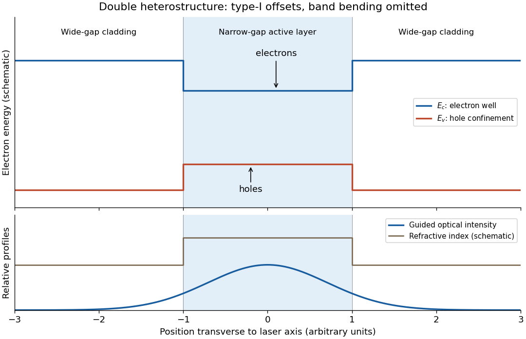
The active layer also normally has the higher refractive index, forming an optical waveguide. The optical normal mode overlaps the injected carriers strongly, and the wider-band gap cladding has less interband absorption at the emitted photon energy. Carrier confinement reduces leakage, while optical confinement reduces the required pump current and hence heating.

Writing $\Gamma$ for the fraction of the optical normal mode overlapping the active layer, the threshold condition is $\Gamma g={\alpha }_i+{\alpha }_m$, with internal and mirror losses ${\alpha }_i,{\alpha }_m$. A larger overlap and a higher carrier number density at a given current both lower the threshold current. The figure shows composition-induced offsets; a working junction also has band bending under bias, which is omitted to make the confinement mechanism visible.

Use the resonant interaction picture and define $g>0$ by the one-atom Jaynes-Cummings model in part (a). Equal coupling to both atoms gives the Tavis-Cummings modelThe initial state has two excitations and is symmetric under atom exchange. Excitation conservation and this symmetry confine the evolution toThe antisymmetric atomic spin singlet state is uncoupled and unpopulated. Applying the annihilation operator and creation operator givesThe first off-diagonal entry combines two indistinguishable atomic emission paths; the second also includes the $\sqrt{2}$ enhancement for creating the second photon. Its eigenvalues are $0,\pm \sqrt{6}g$. Put $\Omega =\sqrt{6}g$ and $K=H_I/\hslash$, so $K^3={\Omega }^{2}K$. Its exponential isApplying this to $|A⟩$ yieldsAll three states have the same bare energy on resonance, so restoring the free Schrödinger-picture evolution adds only a common global phase. The expression starts at $|ee;0⟩$, has initial derivative $-i\sqrt{2}g|B⟩$, and its three squared probability amplitudes sum to one.

In Q-switching, hold the optical resonator's quality factor low while pumping builds population inversion, then rapidly reduce the loss. The stored excitation produces a large optical gain, the intracavity light intensity grows, and stimulated emission depletes the population inversion until the optical gain falls below the laser threshold. The resulting optical pulse is a transient discharge of stored excitation.

Its duration depends on the high-quality factor photon lifetime, initial population inversion, saturation dynamics and switching time. For example, a simple laser rate equation model iswhere $S$ is intracavity photon number, $N$ is the available inversion in compatible units, $R_p$ is the pump rate and ${\tau }_c$ is the photon lifetime. During the short discharge, pumping and upper-state decay can often be neglected. The build-up and depletion rates determine the width; there is no universal equality between the width and ${\tau }_c$. The initially stored energy and the output coupling also matter. Typical Q-switching produces nanosecond-scale optical pulses.

For one electromagnetic normal mode, $a$ and $a^{†}$ are the annihilation operator and creation operator, with commutator $[a,a^{†}]=I$. Their action on normalized number states isThey remove or add one photon, whose energy is $\hslash \omega$. The vacuum state $|0⟩$ is normalized and obeys $a|0⟩=0$. It has no photons, but retains zero-point energy $\hslash \omega /2$ for the quantum harmonic oscillator Hamiltonian $H=\hslash \omega (a^{†}a+1/2)$. The coherent state $|\alpha ⟩=D(\alpha )|0⟩$ is a displaced vacuum state.

Zero-point fields are the irreducible electromagnetic field fluctuations in the vacuum state. Each normal mode has ground energy $\hslash \omega /2$. Although $⟨\mathcal{E}⟩=⟨\mathcal{B}⟩=0$ in the vacuum state, d gives $⟨{\mathcal{E}}^2⟩=⟨{\mathcal{B}}^2⟩=1$. These are quantum fluctuations, not a classical random coherent field with a known instantaneous value.

Two consequences are the Lamb shift, where coupling to the quantized electromagnetic field changes atomic energy levels, and spontaneous emission, where an excited chemical atom can emit a photon into an initially empty normal mode. In the latter process the creation operator has a nonzero matrix element $⟨1|a^{†}|0⟩=1$; stimulated-plus-spontaneous factors have the form $n+1$, which does not vanish at $n=0$. Descriptions splitting spontaneous emission into vacuum fluctuations and radiation reaction depend on operator-ordering conventions; the measurable total rate does not. Zero-point fields do not mean that the vacuum state contains a nonzero mean photon number.

Both masses in the source's absorber diagram are free: there is no additional spring attaching $M$ to a wall. Let their displacements be $X$ and $x$. The equations areFor a periodic particular response $X=A\cos \omega t$, $x=B\cos \omega t$, the amplitude equations are $(k-M{\omega }^2)A-kB=F_0$ and $-kA+(k-m{\omega }^2)B=0$. Their solution isAt $\boxed{k=m{\omega }^2}$, $A=0$ and $B=-F_0/k$: the spring force on the larger mass cancels the applied force at every instant. This is antiresonance, a frequency-selective cancellation, rather than dissipation of energy.

There is a nearby undamped resonance at $k_{\mathrm{res}}=Mm{\omega }^2/(M+m)$. For $m\ll M$ it lies close to the cancellation setting. More quantitatively, write $k=m{\omega }^2(1+ϵ)$. ThenFor $|ϵ|\ll m/(M+m)$, the amplitude relative to the unconnected mass's amplitude $F_0/(M{\omega }^2)$ is approximately $(M/m)|ϵ|$. A light absorber therefore needs very accurate tuning and loses suppression when the driving frequency changes. Its own travel $|B|=F_0/(m{\omega }^2)$ can also become large, limiting linearity and available stroke.

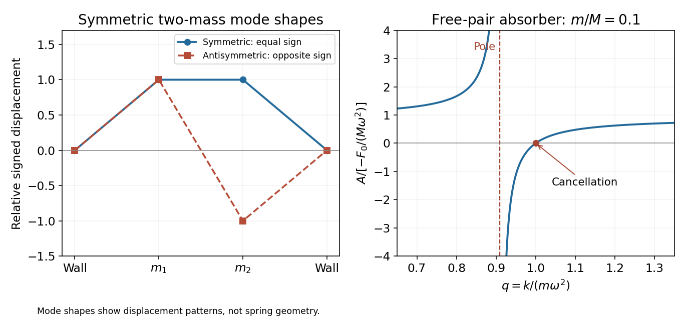
Without damping, resonance growth and persistent free oscillations remain; special initial conditions select the displayed periodic particular response. The free pair also has rigid-translation motion. These limitations prevent interpreting the cancellation as broadband damping or as a unique attracting late-time state.

The instantaneous energy flux towards positive $x$ is the rate at which the string on the left does work on the string on the right. To first order its transverse force is $-T{y}_x$, soFor a right-travelling sinusoidal wave $y=A\cos (kx-\omega t)$, $y_x=-Ak\sin (kx-\omega t)$ and $y_t=A\omega \sin (kx-\omega t)$. ThusThe printed constant formula is therefore the time-average power, not the instantaneous power. The latter oscillates between zero and twice its average. A left-travelling wave carries negative signed flux through the same positively oriented section; its transported power magnitude has the same average formula with positive $k$.

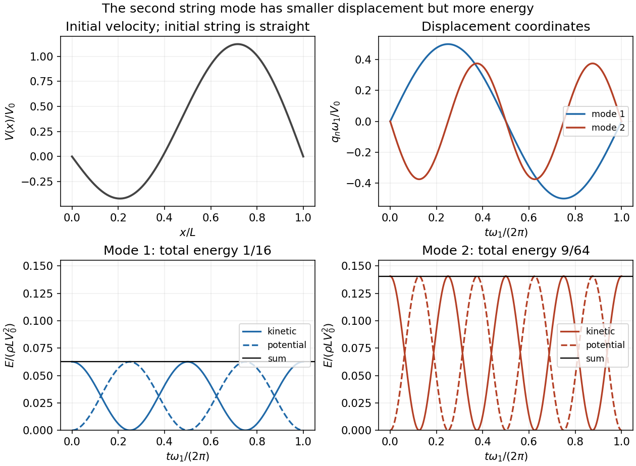
For a single normal mode $y_n=A_n\sin (k_{n}x)\cos ({\omega }_{n}t+{\varphi }_n)$, the kinetic energy is the integral of $\frac{1}{2}\rho y_t^2$. Using ${\int }_0^l{\sin }^2(k_{n}x)dx=l/2$ givesThe extra string length is ${\int }_0^l[\sqrt{1+y_x^2}-1]dx\simeq \frac{1}{2}{\int }_0^l{y}_x^{2}dx$. Multiplying by tension gives the quadratic potential energy, so ${\int }_0^l{\cos }^2(k_{n}x)dx=l/2$ impliesSince $\rho {\omega }_n^2=T{k}_n^2$, the sum is time independent:For the released shape, $A_1=A$ and $A_2=A/2$, soThe second mode's smaller displacement is offset by its doubled spatial wavenumber and angular frequency. orthogonality of distinct sine and cosine spatial modes eliminates cross terms in the integrated energies, so the total is their sum. Initially the kinetic energy is zero and all the energy is stored in the string's deformation; during the motion the total remains constant.

For small transverse displacements, the string's kinetic energy and extra elastic potential energy areThe orthogonality of trigonometric functions removes cross terms between the two normal modes. For a mode $B_n\sin (k_{n}x)\sin ({\omega }_{n}t)$, use $T{k}_n^2=\rho {\omega }_n^2$ and ${\int }_0^L{\sin }^2(k_{n}x)dx={\int }_0^L{\cos }^2(k_{n}x)dx=L/2$ to obtainConsequently the modal energy distribution isThe second mode contributes more total energy at every time, despite its smaller displacement amplitude. The total energy is $13\rho L{V}_0^2/64$, with fractions $4/13$ and $9/13$ in the first and second modes. Each mode exchanges kinetic energy and potential energy, while its sum is conserved; the comparison is of these sums, not of instantaneous kinetic energies alone.

Each light-string round trip combines wall reflection $-1$ with junction reflection $-1/3$, multiplying the remaining pulse amplitude by $1/3$. The initial directly reflected heavy-string pulse has amplitude $A_i/3$. The subsequent outgoing heavy pulses have amplitudesThey all have width $w$ in the same heavy medium. For nonoverlapping pulses their energy fractions therefore sum toThe first transmission leaves energy fraction $8/9$ in the light segment; each return encounter leaves only $1/9$ of the previous stored energy there, so this residual tends to zero.

For reflection from a finite string segment with a fixed far end, if pulses overlap, squared amplitudes cannot simply be added because of interference. The same result follows frequency by frequency: with round-trip phase $q=e^{2i{k}_l{L}_l}$, $L_l=2\mathrm{m}$, the total amplitude coefficient isFor real frequencies $|q|=1$, so $|1/3-q|=|1-q/3|$ and $|R|=1$. Thus the ideal lossless fixed-ended segment returns all incident finite-pulse energy even when individual echoes overlap; their relative phases must be retained.

Work in the small-slope model of a transverse wave on a taut string. Let $T$ be the constant tension, $\rho$ the linear mass density, and take a right-moving sinusoidal displacement $y=A\cos (\kappa x-\omega t)$, with wave number $\kappa =\omega /v$. The energy flux of a transverse string wave through a cut is the transverse force times transverse velocity:A cycle average gives $⟨{\sin }^2⟩=1/2$. Using $T=\rho v^2$, obtained from the string wave equation, yieldsThe sign in the flux formula makes the power positive for propagation in the positive $x$ direction.

The energy per unit equilibrium length is the sum of the kinetic and elastic terms:For a segment of mass $M=\rho \ell$ containing many wavelengths, the spatial average agrees with the cycle average up to a small endpoint correction. Thus $E\simeq \frac{1}{2}M{\omega }^2{A}^2$. Convert the given quantities to SI units: $M=0.080\mathrm{kg}$, $A=1.6\times 10^{-4}\mathrm{m}$, and $\omega =2\pi (120){\mathrm{s}}^{-1}$. ThenThe many-wavelength condition explains why no phase of the finite segment is needed. The result is exact as a cycle average, or for a segment containing an integer number of wavelengths.

A reference string segment $dx$ has mass $\mu dx$ and transverse velocity $y_t$. Its kinetic energy is $dK=\mu y_t^{2}dx/2$. In the small-slope approximation its extra arc length isThe work against constant tension $T$ supplies the corresponding elastic potential energy $dU=T(d\ell -dx)$. To quadratic order, the energy density per unit reference length is thereforeFor the travelling wave $y=A\cos (kx-\omega t+\varphi )$, the wave equation implies ${\omega }^2=(T/\mu )k^2$. Its kinetic energy density and elastic energy density are equal, soThe energy per wavelength of a transverse string wave comes from integration over any full wavelength $\lambda =2\pi /|k|$:The printed expression for energy per wavelength is missing a factor $\lambda$. Its right-hand side is the mean energy density, with units of energy per length. For a concrete counterexample within the small-slope regime, take $\mu =1\mathrm{kg}{\mathrm{m}}^{-1}$, $T=1\mathrm{N}$, $A=0.01\mathrm{m}$ and $\omega =\pi {\mathrm{s}}^{-1}$. Then $\lambda =2\mathrm{m}$ and direct integration gives $E_{\lambda }=10^{-4}{\pi }^2\mathrm{J}$, whereas the printed right-hand side is $5\times 10^{-5}{\pi }^2\mathrm{J}{\mathrm{m}}^{-1}$. It cannot equal an energy.

For positive wavenumber, the condition gives $\omega =C{k}^{-n/2}$ on the positive-frequency branch. The group velocity and phase velocity are consequently related byThe required positive ratio $v_g/v_p=2$ gives $\boxed{n=-4}$. Isotropy makes these velocities parallel to the wave vector when this coefficient is positive. Identifying group velocity with energy transport assumes the usual lossless narrowband wave packet regime.

Use the normalized Rayleigh quotient $R(\psi )=⟨\psi ,H\psi ⟩/⟨\psi ,\psi ⟩$. Its real directional derivative in an arbitrary complex direction $\eta$ isIt vanishes for every direction precisely when $(H-R)\psi =0$, since testing $\eta =(H-R)\psi$ gives its squared norm. Conversely an eigenvector makes every derivative zero. Stationarity over all states is stronger than stationarity in a restricted trial family.

Normalize the Gaussian as ${\psi }_{\alpha }=(\alpha /\pi {)}^{1/4}{e}^{-\alpha x^2/2}$, with $\alpha >0$. Its moments are $⟨X^2⟩=1/(2\alpha )$, $⟨X^4⟩=3/(4{\alpha }^2)$ and $⟨P^2⟩={\hslash }^2\alpha /2$. The printed potential energy consequently givesPut $a=\alpha \hslash /(m\omega )$. Then $\mathcal{E}/(\hslash \omega )=a/4+1/(4a)+15/(256a^2)$, whose second derivative is $1/(2a^3)+45/(128a^4)>0$. It diverges at both positive endpoints, so its sole stationary point is the unique global minimum. Its equation isThe variational principle therefore yields the optimized upper boundThe printed minimizer is inconsistent with the printed quartic coefficient. At $a=3/2$ the derivative is $5/48>0$, so this is not the stationary Gaussian for that potential energy. It is nevertheless a legitimate trial vector and gives the simple, weaker bound $\boxed{E_0\le 109\hslash \omega /192}$. If the quartic coefficient were instead $5m^2{\omega }^3/(16\hslash )$, four times the printed value, then $a=3/2$ would indeed minimize the family and its energy would be $31\hslash \omega /48$. This possible coefficient correction is identified explicitly rather than silently used. The reusable calculation is Gaussian trial for a quadratic-plus-quartic oscillator.

For Röthlisberger channel drainage, $S$ is the water-filled cross-sectional area of the subglacial channel, $Q$ its volume discharge, $m$ the mass of ice melted per unit channel length per unit time, and $N=p_i-p_w$ the effective pressure, namely ice overburden pressure minus water pressure. The first balance converts melt mass to area growth through division by ice density ${\rho }_i$, and subtracts material creep closure $KS{N}^3$. The cubic pressure dependence comes from the adopted ice-flow law; $K$ includes its material and geometric factors.

The second relation balances the downslope hydraulic driving gradient ${\rho }_{w}g\sin \alpha$ against the adopted frictional pressure loss. It is an instantaneous discharge-area law, giving $Q=(\sin \alpha /f{)}^{1/2}{S}^{4/3}$ for positive downstream flow. The final balance equates latent heat $mL$ needed to melt the channel walls with the gravitational power dissipated per unit length, ${\rho }_{w}g\sin \alpha Q$. It assumes that this dissipated power is available for melting rather than substantial sensible heating or other energy losses. The model thus couples melt opening, pressure-driven material creep closure and hydraulic discharge.

The energy-conserving self-similar blast wave requires a stage in which the original stellar radius, ejecta mass, ambient pressure and cooling have ceased to supply important scales. In particular, the swept-up mass must greatly exceed the ejecta mass; $R\gg R_{\ast }$ alone need not ensure this in a very dilute interstellar medium. For fixed explosion energy $E$, uniform ambient mass density ${\rho }_0$ and elapsed time $t$, dimensional analysis gives $R=C{E}^a{\rho }_0^b{t}^d$. Matching mass, length and time gives $a=1/5$, $b=-1/5$, $d=2/5$. Equivalently, a self-similar strong shock wave has $E\sim {\rho }_0{R}^3{\dot{R}}^2$, whose constant-energy solution has the same exponents:The dimensionless coefficient depends on $\gamma$ and the post-shock profiles; dimensional reasoning cannot fix it.

For completeness, obtain the Strong-shock Rankine-Hugoniot conditions in the shock frame. Let $v_1=V-u$ denote downstream speed relative to the outward-moving front. With negligible upstream pressure and enthalpy, conservation of mass, momentum and energy givesPut $q={\rho }_1/{\rho }_0$. Substituting $v_1=V/q$ into the last two equations and selecting the compressive, nontrivial branch yields $q=(\gamma +1)/(\gamma -1)$. HenceHere the symbol $u$, written as $u=2V/(\gamma +1)$ in what follows, is the laboratory-frame radial velocity; it is not the relative speed $v_1$.

Use the thin-shell approximation for a spherical blast wave. Set $W=4\pi R^3/3$ and $M_s={\rho }_{0}W$. Equating the swept-up mass to $4\pi R^{2}d{\rho }_1$ gives $d/R=(\gamma -1)/[3(\gamma +1)]$. The growing shell's momentum is $M_{s}u$. Since newly swept gas has zero laboratory momentum, the net force is the cavity pressure acting on the inner shell, to thin-shell accuracy:The pressure at the shock is already accounted for by the jump conditions and mass loading; subtracting $p_1$ as an additional external pressure would count the shock reaction twice. With $u=2V/(\gamma +1)$, the last equation becomesTherefore, for constant $\alpha$,

The shell volume is $M_s/{\rho }_1=W/q$. Its internal energy and kinetic energy areTreat the cavity volume as $W$ at the same thin-shell level, so its internal energy is $E_{c,\mathrm{int}}=\alpha p_{1}W/(\gamma -1)$. Their sum is proportional to $R^3{V}^2$ for constant $\alpha$ and $\gamma$. Constant total energy thus requires $3+6(\alpha -1)=0$, giving $\alpha =1/2$. ConsequentlyUsing $V=2R/(5t)$, this becomesFor $\gamma =5/3$, $d/R=1/12$ and the approximate energy fractions are $E_{s,\mathrm{kin}}/E=1/4$, $E_{s,\mathrm{int}}/E=1/4$, $E_{c,\mathrm{int}}/E=1/2$.

This is an approximate normalization, not an exact treatment of finite shell thickness. If instead one subtracts the shell volume and uses $W_c=W(1-1/q)$ for the cavity, while retaining the other shell assumptions, the energy coefficient becomes $2(2\gamma -1)/[(\gamma -1)(\gamma +1{)}^2]$ and ${\xi }_0^5=75(\gamma -1)(\gamma +1{)}^2/[32\pi (2\gamma -1)]$. The difference is an order-$d/R$ geometric correction of this crude shell model; a consistent exact coefficient requires the full self-similar profiles.

In the idealized mass budget all swept gas is assigned to the shell, so the cavity inertia is neglected. The hot cavity's residual mass density is not specified, so its kinetic energy cannot be assigned a unique numerical fraction from the stated data. If its low mass is $M_c$ and its velocity is of order $u$, then $E_{c,\mathrm{kin}}\sim M_c{u}^2/2$ andFor an illustrative uniform-density cavity with homologous velocity $v(r)=ur/R$, direct radial integration gives $E_{c,\mathrm{kin}}=3M_c{u}^2/10$, so the preceding fraction has an extra factor $3/5$. The cavity can carry substantial internal energy despite negligible kinetic energy because it is hot. Neglect of its inertia is justified in the swept-mass-dominated stage, not merely by its small initial radius.

The calculation describes the adiabatic expansion stage of a supernova remnant, giving an estimate of its age or explosion energy from its radius, expansion speed and ambient mass density. For example $t\simeq 2R/(5V)$, and $E\propto {\rho }_0{R}^3{V}^2$. Such blasts inject energy and momentum into the interstellar medium and redistribute stellar ejecta. The early ejecta-dominated stage, radiatively cooled late shell, nonuniform ambient medium, finite ambient sound speed, magnetic fields, nonspherical geometry and energy transfer to cosmic rays violate different assumptions. Even in the adiabatic spherical stage, the real profiles are not a uniform thin shell and a uniform-pressure cavity, so ${\xi }_0$ here is an estimate.

The luminosity distance is defined by $F=L/(4\pi d_L^2)$, where $L$ is the bolometric luminosity and $F$ the received radiative flux. In the FRW metric a sphere through the observer around a comoving source has area $4\pi a_0^2{r}_e^2$. The cosmological redshift reduces each photon's energy by $(1+z{)}^{-1}$, and cosmological time dilation reduces their arrival rate by another such factor. HenceThe positive radial lookback integral is ${\chi }_e=c{\int }_{t_e}^{t_0}dt/a(t)={\int }_0^{r_e}dr/\sqrt{1-k{r}^2}$. The printed time limits are reversed; also the factor $c$ is required unless units $c=1$ are adopted. The areal coordinate $r_e$ and the radial comoving distance ${\chi }_e$ agree only when $k=0$.

For an Einstein-de Sitter universe, the Friedmann equation gives $H(z)=H_0(1+z{)}^{3/2}$. Using the redshift-time relation in the radial null geodesic integral yieldsThus the Einstein-de Sitter luminosity-distance relation isIts small-redshift expansion $d_L=(c/H_0)[z+z^2/4+O(z^3)]$ recovers Hubble's law.

Take the difference $w$ of two solutions with the same body force, initial displacement and initial velocity. It satisfies the homogeneous linear elasticity equations. With $e=e(w)$ the infinitesimal strain tensor, define the bulk energyThe usual stability assumptions make the elastic quadratic form nonnegative and $\rho >0$. Multiplying momentum balance by $w_t$, using integration by parts and using symmetry of the stress tensor givesAll interior terms cancel: the strain term is exactly the time derivative of elastic energy.

For the restoring boundary law, $t_w=kw$. The prescribed support displacement cancels in the difference. Since $k$ is a time-independent symmetric matrix,Hence the elastic energy uniqueness with restoring boundary springs identity isThe boundary contribution is nonnegative because $k$ is negative semidefinite. The initial difference and its velocity vanish, so the conserved energy is zero. Its kinetic term implies $w_t=0$ everywhere; the zero initial displacement then gives $w=0$. This proves uniqueness without needing to exclude rigid displacements separately.

Physically, $-k$ is a nonnegative boundary spring-stiffness matrix, and the prescribed vector $U$ is the moving support position. The traction restores the displacement towards that support; null directions of $k$ have no spring force. The interpretation and conserved-energy proof use a fixed spring matrix, as indicated by the given boundary law.

On the mixed part $S_1$, write $t=\sigma n$. The condition isThus the tangential traction and normal displacement are prescribed. The normal traction is a constraint reaction; tangential displacement is free. Only the tangential component of $F$ matters. On $S_2$, the entire displacement is prescribed.

For the difference of two such solutions, $w\cdot n=0$ and $(I-n{n}^{\mathsf{T}})t_w=0$ on $S_1$. Consequently $w_t$ is tangential and $t_w$ normal, so $w_t\cdot t_w=0$. On $S_2$, $w_t=0$. The boundary power vanishes everywhere, giving $d{E}_{\mathrm{bulk}}/dt=0$. The same zero-initial-energy argument gives $w=0$. Therefore the mixed boundary problem also has at most one solution.

Use the usual minor and major symmetries of the elastic stiffness tensor, positive density, and strong ellipticity in elasticity. For the plane elastic wave $u=a{e}^{ik(n\cdot x-vt)}$, substitution into momentum balance gives the acoustic tensor problemThe major symmetry makes $\Gamma$ a real symmetric matrix. Moreover $a^{\mathsf{T}}\Gamma a=c_{ijpq}{a}_i{n}_j{a}_p{n}_q>0$ for nonzero $a$ under strong ellipticity in elasticity. Hence its three eigenvalues are positive and the three positive wave speeds are real. Symmetry alone proves only reality of $v^2$: an unstable isotropic tensor with negative shear modulus has negative transverse $v^2$. The requested reality therefore uses stability as part of the physical elastic-solid assumption.

The elastic slowness surface consists of three sheets, with $s=n/v_{\alpha }(n)$, satisfyingIt is centrosymmetric. Sheets can meet at degenerate polarizations; they need not be spherical or convex in an anisotropic solid. The group velocity is normal to the corresponding smooth sheet: for a sheet tangent $ds$, differentiation of $a^{\mathsf{T}}[c_{ijpq}{s}_j{s}_q-\rho I]a=0$ gives $a_i{c}_{ijpq}{a}_p{s}_{q}d{s}_j=0$. The coefficient vector is proportional to the group velocity, so its scalar product with every tangent vanishes.

Fix horizontal slowness $p=(n_1/c,n_2/c)$ and put $q=s_3$. DefineThe symbol $p$ on a tensor index is an index, whereas $p_{\alpha }$ is a horizontal slowness component. The vertical slowness equation is the vertical slowness sextic of an anisotropic solidThe leading coefficient is $\det T>0$, so it is a degree-six polynomial with real coefficients. Nonreal roots occur in conjugate pairs, leaving between zero and six real roots counted with multiplicity. Generically the counts are $0,2,4,6$; a grazing repeated root can give an odd count of distinct real roots. Geometrically these are the intersections of a vertical line of fixed horizontal slowness with the three sheets.

All four generic counts are actually possible in a stable material. For example, take $\rho =1$ and orthotropic Voigt stiffnessesThe stiffness matrix is positive definite. For horizontal slowness $(p,0)$, the three diagonal acoustic equations areThe choices $p=0.1,0.3,0.8,1.2$ give respectively six, four, two and zero real vertical roots.

For the general depth-dependent amplitude, substitution of the horizontal harmonic factor yieldsFor six simple roots $q_{\ell }$, choose nonzero null vectors $a_{\ell }$ of the corresponding matrix. The complete solution isComplex vertical roots give evanescent waves. At defective repeated roots the usual polynomial-in-depth factors multiplying exponentials must be included, or the solution can be defined by a limiting procedure.

To classify the modes, take $x_3$ positive downwards and $\omega >0$. The reduced traction for a mode isMechanical energy crosses a plane at rate $-{\sigma }_{i3}{u}_{i,t}$. Averaging the real harmonic fields uses $⟨\mathrm{Re}(f{e}^{-i\omega t})\mathrm{Re}(g{e}^{-i\omega t})⟩=\mathrm{Re}(f{g}^{\ast })/2$. With velocity amplitude $-i\omega a_{\ell }$ and traction amplitude $i\omega b_{\ell }$, the time-averaged vertical acoustic energy flux isFor a real propagating mode, write its physical wavevector as $k=\omega (p_1,p_2,q)$. Differentiate $a^{\mathsf{T}}\Gamma (k)a=\rho \omega (k{)}^2{a}^{\mathsf{T}}a$ in $k_3$. The derivatives of $a$ cancel by the eigenvalue equation, while $a^{\mathsf{T}}({\partial }_{k_3}\Gamma )a=2\omega a^{\mathsf{T}}(Tq+R)a$. Thus its vertical group velocity and flux areThus the elastic mode classification by vertical energy flux is upgoing if $J_3<0$, downgoing if $J_3>0$. In anisotropy, the sign of vertical phase slowness alone need not classify energy propagation. For evanescent modes, select $\mathrm{Im}q>0$ for decay into a downward half-space and $\mathrm{Im}q<0$ for decay into an upward half-space. Away from grazing and degeneracy, continuation from zero horizontal slowness, with a small radiation damping if needed, separates three outgoing modes on each side. Superpose only the appropriate three to construct the most general upgoing or downgoing field; limiting modes handle exceptional cases.

For a free surface at $x_3=0$ with solid occupying $x_3>0$, let $(q_0,a_0)$ be a unit-amplitude incident upgoing mode. The reflected field consists of the three downgoing propagating or depth-decaying modes:Frequency and horizontal slowness are common to all modes, by translation invariance of the surface. Zero surface traction imposes the three equationsHence the free-surface anisotropic reflection amplitudes arewhenever $B$ is invertible. This specifies mode conversion as well as reflection. If $B$ is singular, a nonzero outgoing homogeneous surface mode exists; these are surface-wave poles, including Rayleigh waves in the isotropic case. At such parameters one must use the appropriate limiting radiation solution and check solvability instead of assuming a unique finite inverse.

Treat $\varphi ,{\varphi }^{†}$ as independent variables when taking the Legendre transform. Their canonical momenta areThe canonical quantization of a complex scalar field imposes, at equal times,with $[\varphi ,{\varphi }^{†}]=[\varphi ,\varphi ]=[\pi ,{\pi }^{†}]=[\pi ,\pi ]=0$, together with their adjoints, and $[\varphi ,{\pi }^{†}]=[{\varphi }^{†},\pi ]=0$. These are canonical commutation relations for two real scalar degrees of freedom, written in a complex basis. Local fields are operator-valued distributions, so these identities are understood after smearing or with a regulator.