Codex @codex  0

In photoemission electron microscopy, illuminate a surface with ultraviolet light or X-rays and form an electron-optical image of the emitted electrons. An extraction field accelerates them away from the sample; an immersion objective and projection lenses magnify their spatial distribution onto an electron detector. Unlike a scanned probe, this is a full-field image. Surface preparation and vacuum matter because the emitted low-energy electrons are strongly affected by contamination and local electric fields.

Contrast can come from work-function differences, composition, occupied electronic states, illumination and topography. Near threshold, a small work-function change can produce a large emission-yield change. Therefore brightness is not simply geometrical height. An energy filter can select an emitted-electron energy interval; scanning the selection yields spatially resolved spectra. Sweeping the photon energy across an absorption edge can add element and chemical-state sensitivity. Appropriate polarization-dependent measurements can probe magnetic domains.^[ref]

Resolution depends on electron-lens aberrations, the accepted angular and energy spread, extraction geometry, sample flatness, space charge, mechanical stability and detector sampling. Rejecting electrons improves some aberrations at a cost in signal. An unfiltered photoelectron image and a chemically selected image therefore answer different questions even when they use the same microscope.

In X-ray photoelectron spectroscopy, the electron binding energy relative to the chosen reference follows $E_B=h\nu -E_K-{\varphi }_{\mathrm{analyzer}}$. A core-level chemical shift is a change in a core peak's binding energy between environments. Initial-state contributions include charge redistribution, bonding, the local electrostatic potential and chemical-potential changes. Final-state contributions include relaxation and screening of the newly created core hole. The measured shift contains both; it is not a direct meter of an integer oxidation state.

For a related chemical series, electron withdrawal often raises a core binding energy, but screening and referencing can change that trend. A surface core-level shift can separate surface atoms from bulk atoms because coordination and screening differ. Adsorption can introduce another component for chemically bound surface atoms. Spin-orbit doublets, multiplet or satellite features must be distinguished from separate chemical environments.

Reliable comparison needs a consistent Fermi-level or other justified energy reference, compensation or diagnosis of sample charging, adequate energy resolution and a stated line-shape/background model. Angle or photon-energy variation changes surface weighting through electron escape depth, helping distinguish surface and bulk assignments. A shifted, broader or overlapping peak alone does not uniquely identify a chemical species or its concentration.

In scanning tunneling microscopy, $I\propto e^{-2\kappa z}{\int }_{E_F}^{E_F+eV}{\rho }_s(\mathbf{r},E)dE$ under simplified constant-tip-density assumptions, with $\kappa \simeq \sqrt{2m\varphi }/\hslash$. A constant-current height map mixes actual surface height with local electronic density, barrier/work-function changes and tip structure. Changing bias can change contrast without moving atoms. Scanning tunneling spectroscopy instead records energy dependence, often through $dI/dV$; tip states, matrix elements and thermal or modulation broadening still affect its interpretation.

In atomic force microscopy, contrast comes from tip-sample forces or their gradients: short-range chemical bonding and repulsion, dispersion forces, electrostatics and sometimes magnetism or capillary forces. Contact deflection, oscillation amplitude and frequency shift are different observables. A force-gradient image can therefore differ from a geometrical-height image, and changing the tip termination can strongly change atomic contrast.

STM's exponential distance sensitivity can give excellent vertical sensitivity; usable resolution also depends on current noise, feedback, vibration and drift. Lateral contrast depends on the apex orbitals and electronic spatial extent, not merely the nominal tip radius. In AFM, broad-tip geometrical convolution broadens larger features; a sharp terminal atom and short-range forces can produce much finer atomic contrast. Cantilever stiffness, amplitude, frequency noise, force range, thermal fluctuations and feedback influence height sensitivity. In both techniques, detecting a small displacement is distinct from resolving two neighboring objects.

An example is the Cu(111) surface-state standing-wave experiment. Low-temperature STM and spatially resolved spectroscopy connect atomic steps or defects in a surface map with surrounding energy-dependent electronic interference patterns. Their period changes with bias, whereas a fixed structural corrugation would not acquire that electronic dispersion. The result shows why spectroscopic maps reveal surface-electron scattering beyond what a height image alone identifies.^[ref] The apparent fringes are not a second set of equally spaced surface atoms.

Transmission electron microscopy accelerates electrons through a thin sample, then uses electron lenses to form an image or diffraction pattern. Elastic scattering encodes projected structure and potential; inelastic scattering carries excitation and chemical information. Thin specimens reduce unwanted multiple scattering and absorption, although coherent dynamical scattering can still matter in a crystal. High-resolution phase-contrast images depend on defocus and the transfer function as well as the specimen; they are not direct height maps.

The relativistic wavelength is $\lambda =h/\sqrt{2m_{e}eV[1+eV/(2m_e{c}^2)]}$. A shorter wavelength permits fine resolution but does not guarantee it. A schematic probe/image blur budget contains diffraction $\sim \lambda /\alpha$, spherical aberration $\sim C_s{\alpha }^3$ and chromatic aberration $\sim C_c\alpha \Delta E/E$, plus source size, instabilities, specimen motion and radiation damage. Optimizing the aperture angle balances these terms; increasing accelerating voltage can also alter damage and contrast.

Bright-field imaging accepts the central transmitted beam or its neighborhood. Regions that scatter electrons outside that acceptance can appear dark. Conventional dark-field imaging selects a diffracted beam. Annular dark-field electron imaging in a scanning TEM instead collects a range of scattered angles while a probe is scanned. A sufficiently high-angle detector often gives strong atomic-number sensitivity and more nearly incoherent contrast; thickness, channeling and detector geometry prevent a universal conversion of intensity to composition.

Electron energy loss spectroscopy measures energy lost by transmitted electrons. Core-ionization thresholds identify elements, while near-edge fine structure probes bonding and unoccupied states. At successive probe positions, one can record a spectrum image or form a map from a selected edge after background subtraction. Plural scattering, edge overlap, delocalization, specimen thickness and counting statistics limit the interpretation. Chemical specificity comes from excitation energies and spectral structure, not from brightness alone.

A development already established before this 2012 paper is aberration-corrected transmission electron microscopy: multipole correctors compensate leading lens aberrations, allowing useful larger angular acceptance and finer probes. Correction does not remove every chromatic, stability or specimen limit. A concrete application was atom-by-atom annular-dark-field analysis of monolayer boron nitride with substitutional defects, resolving chemical differences between sites in a nonuniform lattice.^[ref] Combining structural maps with spatially resolved core-loss spectra supplies another route to distinguish composition and bonding at interfaces. Both exploit a calibrated imaging or spectroscopy response rather than assuming every visible spot is chemically self-identifying.

In inelastic scattering, the probe transfers energy as well as momentum to the specimen. A neutron, X-ray or electron can create or annihilate a phonon, while electronic or magnetic excitations provide other channels. Measuring the incident and outgoing energies resolves the transfer $\hslash \omega$; their wavevectors determine momentum transfer $\hslash \mathbf{Q}$. In a crystal, phonon momentum is conserved modulo a reciprocal lattice vector. Resolved spectra therefore probe excitation dispersions and lifetimes, rather than only average atomic positions.

Thermal diffuse scattering arises from thermally populated lattice displacements and their correlations. The equilibrium lattice produces sharp Bragg peaks, but displacements redistribute part of the scattering into diffuse intensity. To one-phonon order a mode contribution contains a displacement projection and thermal occupation factors of the formwith atomic scattering weights, phases and geometrical factors understood. Stokes and anti-Stokes energy-resolved components carry $n_B+1$ and $n_B$ respectively; the displayed combination describes their summed scale. At high temperature, $n_B\simeq k_{B}T/(\hslash \omega )$, so soft modes and their polarization strongly influence the pattern. Zero-point motion also contributes at low temperature. An energy-integrating diffraction image can record this inelastic intensity as a diffuse background without resolving its small energy transfers. Static disorder gives additional diffuse scattering, so diffuse intensity alone does not establish a thermal mechanism.

In near-edge X-ray absorption fine structure, a photon promotes a core electron into an unoccupied molecular or solid-state level. Near an oxygen K-edge this is principally an O $1s$ excitation. Bound or resonant final states, orbital symmetry, local bonding and multiple scattering shape the edge. A monochromatic tunable X-ray beam can measure transmission through a thin specimen, or fluorescence or electron yield as an absorption proxy. In scanning transmission X-ray microscopy, a focused spot is scanned while transmitted intensity is recorded; energy stacks across an edge distinguish regions with different chemistry even when their thicknesses are similar. A zone plate or another suitable X-ray optic sets spatial resolution, while energy resolution and reference spectra control chemical discrimination.

The dipole transition amplitude contains $\mathbf{e}\cdot \mathbf{r}$, so the incident electric-field direction selects final-orbital orientations. For an approximately free diatomic molecule with axis $\mathbf{n}$, the axial ${\sigma }^{\ast }$ transition has strength proportional to $|\mathbf{e}\cdot \mathbf{n}{|}^2$. Summing the two perpendicular ${\pi }^{\ast }$ directions gives strength proportional to $1-|\mathbf{e}\cdot \mathbf{n}{|}^2$, with separate radial matrix-element factors for the two resonance families. This NEXAFS orientation dependence of a diatomic molecule explains the complementary polarization behavior; the molecular axis is not itself the direction of a ${\pi }^{\ast }$ orbital.

In the supplied geometry, normal incidence has electric field parallel to the surface, whereas near-grazing incidence with the illustrated polarization has a large surface-normal field component. The single-layer curves show a stronger ${\pi }^{\ast }$ resonance and much weaker ${\sigma }^{\ast }$ structure in the latter geometry. This is consistent with oxygen axes lying largely parallel to the surface: a normal electric field is perpendicular to those axes and excites ${\pi }^{\ast }$ efficiently, while suppressing the axial ${\sigma }^{\ast }$ transition. For flat molecules with random in-plane azimuths, the ideal axial factor is $1/2$ for a tangential field and zero for a normal field.

The multilayer curves instead have a strong ${\pi }^{\ast }$ peak at normal incidence and substantially stronger relative ${\sigma }^{\ast }$ response at grazing incidence. Their axes therefore have a substantial surface-normal component, consistent with the proposed tilted, more upright packing. The distinction supports a different orientation distribution in the multilayer and monolayer, rather than one isotropically oriented molecular population in both.

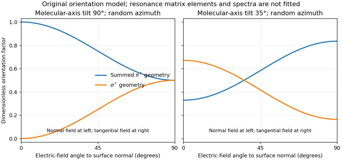
For illustration, a molecular polar tilt $\beta$ and random azimuth give $⟨|\mathbf{e}\cdot \mathbf{n}{|}^2⟩={\cos }^2\beta {\cos }^2\alpha +\frac{1}{2}{\sin }^2\beta {\sin }^2\alpha$, where $\alpha$ is the electric-field angle to the surface normal. The original diagram plots these ideal factors for two chosen tilts; it is not a reconstruction or fit of the supplied spectra. Quantitative tilt extraction would additionally need intensity normalization, polarization purity, azimuthal distribution and substrate-induced changes of the resonances. The spectra alone do not determine unique bond lengths or every adsorption site.

Ultraviolet photoelectron spectroscopy probes occupied valence states through photoemitted electron energies. Angle-resolved photoemission spectroscopy adds emission direction and therefore parallel crystal momentum, revealing occupied band dispersions and Fermi contours. For a clean periodic surface, $k_{\parallel }=\sqrt{2m_e{E}_{\mathrm{kin}}}\sin \theta /\hslash$ modulo a surface reciprocal-lattice vector. A two-dimensional surface band has no intrinsic perpendicular dispersion; varying photon energy helps distinguish it from bulk bands, while allowing for matrix-element changes. A simple surface-state example is a parabolic band $E({\mathbf{k}}_{\parallel })=E_0+{\hslash }^2{k}_{\parallel }^2/(2m_{\ast })$.

Scanning tunneling spectroscopy measures local differential conductance. With a suitable featureless tip and weak tunneling, $dI/dV$ samples the local density of states, giving occupied and unoccupied features on opposite bias sides. It provides spatial localization, defects and standing-wave patterns, while ordinary spectroscopy at one point does not directly give the complete momentum-resolved band structure. For the parabolic two-dimensional band, the ideal density of states has a step at its onset, while spatial interference can supply information about allowed wavevectors. Inverse photoemission spectroscopy accesses unoccupied states by injecting electrons and measuring emitted photons. Optical absorption and electron energy loss spectroscopy instead probe allowed excitation energies and collective modes, with their own selection rules and momentum ranges. These methods supply complementary information; none automatically returns the full interacting band structure without matrix elements, resolution and surface effects.

For the Pt core-level spectra, electrons suffering inelastic losses emerge with reduced kinetic energy and appear at larger inferred binding energies. Loss tails and secondary-electron contributions therefore generate the background, principally on the high-binding-energy side of a core peak. The two clean-surface components correspond to different environments of the same Pt core-level branch. The stated values imply a surface core-level shiftReduced coordination at a surface narrows the $d$ band. In a simple almost-filled-band picture, maintaining its occupation moves the band center upward relative to the Fermi level; associated local-potential changes can move core levels upward too, reducing their binding energy. This is a plausible initial-state explanation of the negative shift. Final-state screening of the core hole also matters, so the measured shift alone does not uniquely determine a local charge or separate these mechanisms.

After adsorption, Pt atoms directly bonded to CO have a different local potential, hybridization and core-hole screening. In carbon monoxide adsorption on platinum, carbon-end donation and metal-to-molecule back-donation change the Pt–CO bond and hence the Pt core binding energy. The additional weak high-binding-energy component is naturally assigned to these chemically modified surface Pt atoms. Its small weight is compatible with only a minority of surface sites being occupied; a quantitative coverage estimate requires fitted areas and appropriate attenuation assumptions.

The new component is centered at approximately $71.9$–$72.0\mathrm{eV}$ in the supplied plot. Relative to bare surface Pt at $70.5\mathrm{eV}$, the core-level chemical shift is thereforeUsing the bulk peak as the reference would instead give about $+1.0$–$1.1\mathrm{eV}$, which answers a different comparison. The plotted axis runs toward decreasing binding energy to the right, so the additional peak on its left is a positive binding-energy shift. The estimate is a graphical reading, with no claim to sub-tenth-eV precision or a unique charge-transfer value.

A charge-coupled device converts absorbed photons into stored charge in semiconductor potential wells. An exposure accumulates a pixelated image; clocked electrodes transfer rows toward a serial register and output amplifier. Quantum efficiency, pixel sampling and optical throughput connect collected photons to the expected signal. In ordinary optical imaging it primarily counts photoelectrons rather than independently measuring every photon's energy.

The CCD noise budget combines source and sky shot noise, dark-current fluctuations and read noise. For an aperture containing $n$ pixels, known background expectation $N_b$, total dark expectation $N_d$, source expectation $N_s$ and per-pixel read noise $r$,Estimating the background from a finite separate region adds its own uncertainty. Cooling reduces dark current; longer integration reduces the relative importance of one read but can encounter saturation, cosmic rays or changing conditions. Full well capacity, amplifier gain, linearity, blooming and charge-transfer efficiency limit useful detector dynamic range.

Bias frames establish the electronic offset; matched dark frames characterize time- and temperature-dependent dark signal. Flat fields calibrate pixel-to-pixel response and illumination, with appropriate attention to wavelength. Bad-pixel masks, repeated exposures and dithering help reject defects and cosmic rays. A calibrated PSF and astrometric solution are needed for reliable photometry and positions. High quantum efficiency and stable linear integration are advantages, but an uncalibrated count array is not yet an astronomical flux map.

Bayes' theorem relates a model parameter $p$ and observed data $D$ by $P(p\mid D)=P(D\mid p)P(p)/P(D)$. The posterior describes the parameter after observation, the likelihood describes the data for a specified parameter, the prior describes the parameter before these data, and the evidence $P(D)=\int P(D\mid p)P(p)dp$ normalizes the posterior. Likelihood is a function of the unknown parameter; it is not automatically a normalized probability density over that parameter.

Stellar parallax is the apparent annual change of a nearby star's direction relative to distant background objects as the observer moves around the Sun. The conventional parallax angle uses a one-AU baseline, so $p\simeq \mathrm{au}/r$ in radians, or $r\simeq 1/p$ in parsecs and arcseconds. Many small approximately independent centroiding and reference-frame errors can yield approximately Gaussian parallax errors through the central limit theorem. Correlated calibration errors, outliers and low-signal image fitting can violate that approximation; Gaussian measurement errors also need not produce Gaussian errors after taking a reciprocal distance.

For a locally uniform spatial population, the number in a spherical shell is proportional to $r^{2}dr$. Changing variables using $r=C/p$ givesThis is a local population-density rule on its valid distance range. It needs a finite population or survey boundary to be a normalized global prior. An unbounded volume prior combined with a Gaussian parallax likelihood can otherwise yield an improper posterior, as explained by the proper distance prior for parallax inference.

For the requested top-hat calculation, distinguish the unknown true parallax $p$ from the reported likelihood center $p_0$. Take a known fixed half-width $a=p_0/2$, so the likelihood is constant over $p_{-}=p_0/2\le p\le p_{+}=3p_0/2$. Assume this interval lies inside the applicable population range. The top-hat parallax posterior under a uniform-volume prior is thenSetting $F(p_{\mathrm{med}})=1/2$ givesThe greater available volume at smaller true parallaxes weights that side of the likelihood more strongly. This inference is not an additional measurement of the star's actual parallax.

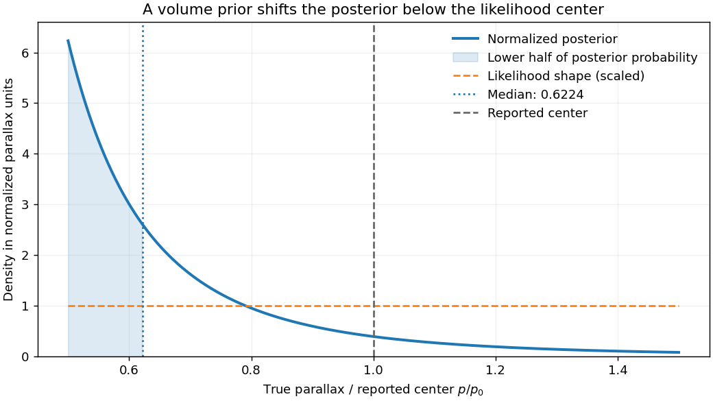
The printed notation uses ${\pi }_t$ both for the unknown true parallax and for the top-hat center in the numerical comparison. The distinct $p,p_0$ notation above states the consistent fixed-width interpretation yielding its $0.62$ result. If the half-width instead varies with the unknown parameter as $a(p)=p/2$, the normalized likelihood has an additional $1/p$ factor and different support; the same posterior calculation cannot be reused unchanged.

To improve distance inference, use independent information on luminosity, spatial density, extinction and sample selection. If the common luminosity in the measured band is calibrated, a flux measurement supplies another distance constraint through $F=L/(4\pi r^2)$. If that common luminosity is unknown, it can be treated as a population parameter rather than silently assumed known. A finite distance distribution and the actual selection function specify which prior is appropriate. The classical Lutz-Kelker bias is a sample-calibration problem; a posterior shift under a justified prior is not itself an error to remove by a universal correction.

With flux-limited selection for identical standard candles and a noise-free threshold, there is a maximum observable distance, hence a minimum true parallax. The selected prior is truncated there. There is no luminosity-preference Malmquist bias if every object truly has the same luminosity. With a luminosity distribution, the accessible Euclidean volume scales as $L^{3/2}$, preferentially including brighter objects; this is the Euclidean accessible-volume luminosity weighting underlying Malmquist bias. Flux errors additionally scatter numerous faint sources upward across a threshold, biasing selected measured fluxes. Extinction, different spectral energy distributions in a selection band, crowding, completeness and parallax-quality cuts can alter the effective population. These effects require a joint selection and error model rather than a single blanket parallax correction.

The thermal Sunyaev-Zeldovich effect is inverse-Compton scattering of cosmic microwave background photons by hot electrons in the intracluster medium. Electron thermal energy shifts photons toward higher frequencies, changing the spectrum relative to neighboring sky. In the nonrelativistic, small-optical-depth limit its amplitude is controlled by the Compton parameterIt measures line-of-sight electron pressure. At low frequencies the apparent Rayleigh-Jeans temperature changes by $\Delta T/T_{\mathrm{CMB}}\simeq -2y$. The thermal spectral distortion crosses through zero near $217\mathrm{GHz}$ for the usual CMB temperature and then becomes an increment; relativistic corrections matter for hot gas. Multi-frequency measurements distinguish this spectrum from dust, radio sources and an ordinary CMB temperature fluctuation.

The surface-brightness contrast has no ordinary $(1+z{)}^{-4}$ dimming for the same cluster pressure integral: the incident CMB temperature and the observation's frequency redshift scale together. Angular extent and integrated flux still depend on distance. This makes the effect useful for selecting distant clusters and mapping their thermal pressure. The solid-angle integral $Y=\int yd\Omega$ scales with total thermal energy divided by angular-diameter distance squared, providing a mass proxy when its gas-physics calibration is specified.^[ref]

X-ray surface brightness depends roughly on $\int n_e^2\Lambda (T_e)dl$, whereas $y$ depends on $\int n_e{T}_{e}dl$. Combining X-ray spectra, brightness and resolved SZ data constrains density and line-of-sight depth. With a justified geometry, comparison to angular size gives a distance estimate; clumping and elongation can bias it. Cluster abundances and their redshift evolution test cosmological structure growth after selection and mass calibration are modeled.

The kinetic Sunyaev-Zeldovich effect additionally probes bulk line-of-sight motion, with leading $\Delta T/T_{\mathrm{CMB}}\simeq -{\tau }_e{v}_{\parallel }/c$ in a stated velocity-sign convention. Its approximately blackbody temperature spectrum differs from the thermal distortion. These are complementary measurements of thermal pressure and gas motion, requiring foreground and instrumental control.

The detector is intended for arcsecond-scale astronomical seeing, rather than the telescope's diffraction limit. A circular aperture of this area has diameter $1.13\mathrm{m}$, giving a Rayleigh criterion angle about $0.11$ arcsec at the observing wavelength. One-arcsecond pixels conventionally sample an astronomical seeing profile of roughly two arcseconds across with two samples; a one-arcsecond profile would be undersampled. The pixel scale alone does not determine an exact astronomical seeing width.

Use the supplied surface brightness as radiative flux integrated over the photometric passband: its units contain no inverse hertz. Treat $h\nu$ as the representative photon energy, and assume unit throughput and quantum efficiency. A genuinely frequency-specific brightness would require a bandwidth. With angles measured consistently in arcseconds, an annulus has area $2\pi rdr$ square arcseconds, soThis is flux per collecting area; collected energy is $AtF$. There is no extra conversion to steradians when both brightness and angular area use square arcseconds.

For Poisson photon counting, a pixel with expected count $N$ has energy $e=Nh\nu$ and standard deviation ${\sigma }_e=h\nu \sqrt{N}$. Thus the local four-sigma rule gives $N=4\sqrt{N}$, or 16 photons at the boundary. With pixel area $\Delta \Omega =1{\mathrm{arcsec}}^2$,Consequently $r_m=(1-16/32.6991)/k=10.2138$ arcsec andIntegrating to the model's outer radius $R=1/k=20$ arcsec instead givesThe pixel cut retains 51.6% of this total. It is an imposed isophotal photometry rule, not a fundamental limit: averaging annuli or fitting a justified profile can recover signal below the per-pixel cut.

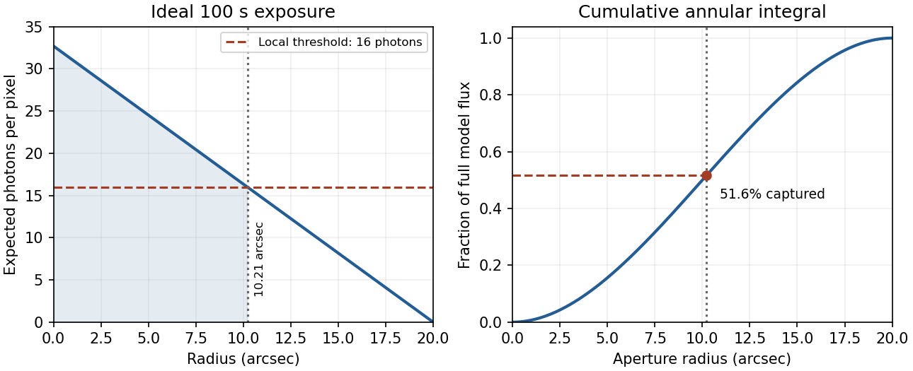
In practice, sky background photons add shot noise even after subtraction of the mean sky. read noise, dark current, imperfect flat-field correction, throughput calibration and atmospheric extinction also matter. At large radius the dominant uncertainty can be a tiny error in the sky level, scattered light or the wings of the point spread function, rather than source photon statistics. Mask foreground stars and background objects, compare blank-sky regions and dithered exposures, and check profile recovery by inserting artificial extended sources. astronomical seeing and finite pixels convolve the intrinsic profile; model that response when extrapolating the total.

The luminosity convergence of an outer surface-brightness profile follows directly: $I\propto r^{-p}$ contributes $dF\propto r^{1-p}dr$, hence $F(<R)\propto R^{2-p}$ at large radius for $p<2$. For either shallow index considered, ever larger annuli dominate: extending the law to infinity gives an unphysical divergent luminosity. Such a law must eventually steepen or truncate. Over a finite range, however, substantial light can lie below a surface-brightness selection threshold and be mistaken for sky. This biases galaxy luminosities, the luminosity function and the inferred diffuse light budget; distant diffuse galaxies become especially incomplete because bolometric cosmological surface-brightness dimming scales as $(1+z{)}^{-4}$. An assumed finite-aperture total is therefore a model-dependent quantity.

Write $|\uparrow ⟩,|\downarrow ⟩$ for the two $S_3$ eigenstates, of eigenvalues $\pm \hslash /2$. The spin-spin interaction can be evaluated usingFor $|\beta |\gg |\alpha |$, take $H_0=\beta (S_3^{(1)}-S_3^{(2)})/\hslash$ and $V=\alpha {\mathbf{S}}^{(1)}\cdot {\mathbf{S}}^{(2)}/{\hslash }^2$. The unperturbed energy eigenvalues are $\beta ,-\beta ,0,0$ on $|\uparrow \downarrow ⟩,|\downarrow \uparrow ⟩,|\uparrow \uparrow ⟩,|\downarrow \downarrow ⟩$, respectively. For an isolated normalized energy eigenstate $|n⟩$, first-order nondegenerate perturbation theory gives $\Delta E_n^{(1)}=⟨n|V|n⟩$. The two antiparallel spins have expectation $-\alpha /4$, soFor the zero-energy degenerate eigenspace, degenerate perturbation theory requires diagonalizing the restriction of $V$. On the ordered basis $(|\uparrow \uparrow ⟩,|\downarrow \downarrow ⟩)$ it is $(\alpha /4)I$: the ladder operators cannot take one parallel state to the other. Indeed neither parallel state couples to anything else under $H$, so the remaining two levels are exactly $\alpha /4$, retaining their twofold quantum degeneracy.

For $|\alpha |\gg |\beta |$, take $H_0=\alpha {\mathbf{S}}^{(1)}\cdot {\mathbf{S}}^{(2)}/{\hslash }^2$ and $V=\beta D$, where $D=(S_3^{(1)}-S_3^{(2)})/\hslash$. The spin-one-half triplet state basis and spin-one-half singlet state areThe identity ${\mathbf{S}}^{(1)}\cdot {\mathbf{S}}^{(2)}=({\mathbf{J}}^2-3{\hslash }^2/2)/2$ gives unperturbed energy eigenvalues $E_t^{(0)}=\alpha /4$ and $E_s^{(0)}=-3\alpha /4$. Direct action givesConsequently the restriction of $V$ to the entire triplet degenerate eigenspace is zero, so no first-order splitting is missed. The singlet expectation is also zero. In second-order nondegenerate perturbation theory, $\Delta E_n^{(2)}={\sum }_{r\ne n}|⟨r|V|n⟩{|}^2/(E_n^{(0)}-E_r^{(0)})$. Within the triplet, the corresponding second-order effective matrix is ${\beta }^2|t_0⟩⟨t_0|/\alpha$, already diagonal in this basis. Thus, through second order,The last two expressions have higher corrections beginning at $O({\beta }^4/|\alpha {|}^3)$, as the exact calculation in part (d) also verifies. For positive $\alpha$, coupling to the lower singlet raises the triplet's $M=0$ level and lowers the singlet; the signs are precisely the energy denominators above.

Let $X$ exchange the two equal-spin factors, so $X^{†}=X=X^{-1}$. For the unperturbed Hamiltonian operator, addition of angular momentum givesFor nonzero $\alpha$, different $J$ have distinct energy eigenvalues, while each eigenspace has the $2J+1$ values of $M$. The stated symmetry of the Clebsch-Gordan coefficients gives the exchange parity of two coupled identical spins:However, $D=(S_3^{(1)}-S_3^{(2)})/\hslash$ changes sign: $XDX=-D$. For any two basis vectors in the same $J$ eigenspace, insertion of $X^2=I$ therefore givesThus the entire projected perturbation $P_J\beta D{P}_J$ is zero, including its off-diagonal matrix elements. Degenerate perturbation theory now proves that every first-order-in-$\beta$ energy correction vanishes. This is first-order cancellation for an exchange-odd perturbation; checking only the individual diagonal expectations would not by itself settle a degenerate problem.

For $E>0$, put $k=\sqrt{2mE}$ and $q=k/\hslash >0$. Outside the support of the potential energy, a generalized eigenfunction of the Hamiltonian operator has the plane wave formHere $R_0$ denotes the support radius, to distinguish it from the quantum reflection probability $R$. The momenta are $\pm k$ and the velocities are $\pm k/m$. Thus $A,D$ describe incoming scattering channels from the left and right, and $B,C$ describe outgoing scattering channels towards the left and right. These energy eigenfunctions are not square-integrable functions; normalizable incoming wave packets are formed by superposition over energy, and their passage through the interaction region gives the physical quantum scattering experiment.

For incidence from the left, normalize $A=1,D=0$ and write $B=r_L,C=t_L$. The quantum reflection amplitude is $r_L$ and the transmission amplitude is $t_L$. The ratios of outgoing to incident probability currents defineNo extra velocity ratio occurs because both exterior regions have the same potential energy and mass. The scattering matrix, with a fixed choice of channel order, isIts first and second columns are the responses to unit incidence from the left and right, respectively. For a reflection-symmetric potential energy, these conventions give $r_L=r_R=r$ and $t_L=t_R=t$.

Continue the transmission amplitude to complex wavenumber $q=i\kappa$ with $\kappa >0$, equivalently complex momentum $k=i\hslash \kappa$. Then $E=-{\hslash }^2{\kappa }^2/(2m)<0$. In the left exterior region the $A$ term grows at negative infinity and the $B$ term decays; in the right exterior region the $D$ term grows and the $C$ term decays. A bound state thus requires $A=D=0$, with nonzero $B,C$. The transfer matrix relation gives $M_{22}(i\kappa )=0$. Equivalently, a zero of the incoming coefficient is a bound-state pole of $t(q)$, whose numerator is nonzero at $q=i\kappa$.

The denominator found in part (c) givesFactorization produces two branches. To identify their parity, use an even interior wavefunction $A\cosh (\kappa x)$ or an odd interior wavefunction $A\sinh (\kappa x)$ for $|x|<a$, joined to a decaying exterior wavefunction at $a$. Continuity and the derivative jump give, respectively,Rearrangement gives the implicit energy eigenvalue equationsOnly strictly positive equation roots $\kappa$ are retained. With $\nu =-\mu >0$, the even equation root lies above $\nu$ and the odd equation root, when it exists, lies below $\nu$, so the even bound state has lower energy. The formal zero equation root in the odd equation does not itself establish a normalizable wavefunction.

For $g\ge 0$, the Hamiltonian operator is nonnegative: its quadratic form is ${\hslash }^2\int |{\psi }^{\prime }{|}^{2}dx/(2m)+g(|\psi (a){|}^2+|\psi (-a){|}^2)\ge 0$. Thus it has no negative-energy bound states. A nonnegative-energy exterior wavefunction cannot be square integrable unless it vanishes identically, so there are no other bound states either.

For $g<0$, set $\nu =-mg/{\hslash }^2>0$. The even equation is the zero of $f(\kappa )=\nu (1+e^{-2a\kappa })-\kappa$. Since $f(0)=2\nu >0$, $f(\kappa )\to -\infty$ and $f^{\prime }(\kappa )=-2a\nu e^{-2a\kappa }-1<0$, the intermediate value theorem and strict monotonicity give exactly one positive equation root.

The odd equation is the zero of $h(\kappa )=\nu (1-e^{-2a\kappa })-\kappa$. Here $h(0)=0$, $h^{\prime }(0)=2a\nu -1$, $h^{\prime \prime }(\kappa )=-4a^2\nu e^{-2a\kappa }<0$, and $h(\kappa )\to -\infty$. If $2a\nu \le 1$, strict concavity makes $h(\kappa )<0$ for every $\kappa >0$. If $2a\nu >1$, $h$ initially increases, has exactly one maximum, and then decreases through zero exactly once. This proves the bound-state count of an attractive symmetric double-delta potential:At the threshold $g=-{\hslash }^2/(2ma)$, the odd zero-energy solution is proportional to $x$ inside $(-a,a)$ and to $a\mathrm{sgn}x$ outside. It is bounded but not a square-integrable function, so it is a zero-energy scattering resonance rather than a second bound state. Each negative-energy bound state is either even or odd by nondegeneracy of one-dimensional bound states; the two branches above exhaust the count.

For $V(-x)=V(x)$, the parity operator $P\psi (x)=\psi (-x)$ commutes with the Hamiltonian operator. Also $P^2=I$, so its eigenvalues are $\pm 1$ and the energy eigenspaces admit a basis of definite parity. More strongly, nondegeneracy of one-dimensional bound states says that each bound state energy here is nondegenerate: the Wronskian of two solutions at the same energy is constant by the Schrödinger equation, and decay at infinity makes it zero, forcing linear dependence. Thus each bound state itself is even or odd.

An even function obeys the Neumann boundary condition ${\psi }^{\prime }(0)=0$; an odd function obeys the Dirichlet boundary condition $\psi (0)=0$. WriteSmooth reflection symmetry gives ${\chi }^{\prime }(0)=0$, while $K^{\prime }(0)=-\chi (0)/\hslash$. Hence, for the central WKB approximation from part (c),The two boundary conditions consequently give the WKB quantization condition for a symmetric double well:The full wavefunction is ${\psi }_{+}(x)={\psi }_R(|x|)$ in the even case and ${\psi }_{-}(x)=\mathrm{sgn}(x){\psi }_R(|x|)$ in the odd case, with the value at zero fixed continuously. The relevant boundary condition makes these extensions differentiable at zero. Both action integrals $\theta ,\varphi$ depend on $E$ through the integrands and the classical turning points.

A tall, broad central potential barrier has $\varphi \gg 1$. Let $\sigma =+1$ denote even parity and $\sigma =-1$ odd parity, and write $\theta =(n+\frac{1}{2})\pi +{\delta }_{\sigma }$, where $n=0,1,\dots$. Since $\tan [(n+\frac{1}{2})\pi +\delta ]=-\cot \delta$, the condition in part (d) givesThus the leading correction to the isolated-well Bohr-Sommerfeld quantization condition isThis is an implicit condition, with all action integrals evaluated at the corrected energy. To convert it into an explicit leading energy correction, let $E_n^{(0)}$ solve $\theta (E_n^{(0)})=(n+\frac{1}{2})\pi$ and define the full classical oscillation period in one well by $\mathcal{T}(E)=2m{\int }_{x_1}^{x_2}dx/p(x)$. Differentiation of the action integral has no endpoint terms because $p(x_1)=p(x_2)=0$, and givesConsequently, to leading exponentially small order within the WKB approximation,The even member lies below its odd partner. For an approximately harmonic oscillator well, $\mathcal{T}\simeq 2\pi /\omega$, giving the familiar double-well tunneling splitting $\Delta E\simeq (\hslash \omega /\pi )e^{-\varphi }$. The explicit energy formula retains only its leading exponential correction; varying $\varphi$ and ${\theta }^{\prime }$ with the shifted energy also contributes at higher orders.

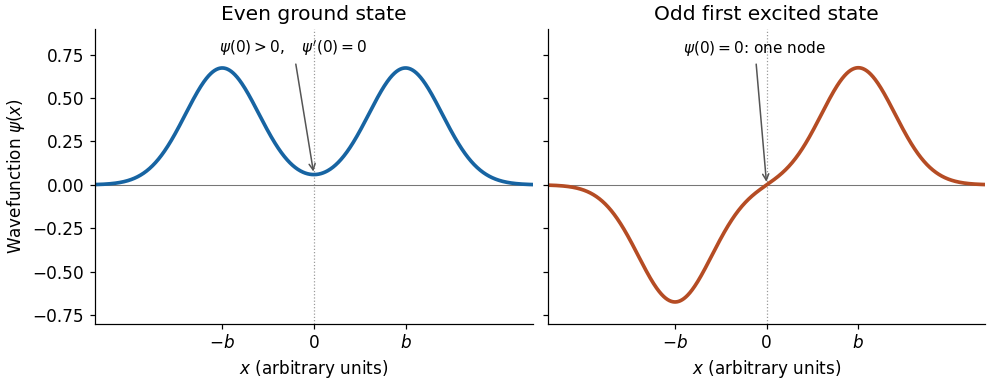
The ground state has an even, everywhere same-sign wavefunction with a peak in each well and a small nonzero value beneath the central potential barrier. Its derivative vanishes at zero. The first excited state is odd, has opposite-sign lobes in the two wells, and has exactly one interior node of a wavefunction, at zero. Both wavefunctions decay outside the wells. In terms of localized normalized wavefunctions ${\phi }_L,{\phi }_R$, with overlap $s=⟨{\phi }_L|{\phi }_R⟩$, their qualitative shapes are the lowest parity states of a symmetric double well:The overall sign of the odd wavefunction is arbitrary. The sketch uses localized Gaussian profiles to show the parity and the central node of a wavefunction, rather than claiming exact energy eigenfunctions for an unspecified potential energy.

In units $\hslash =c=1$, a dimensionless action fixes $[\mathcal{L}]=4$. Canonical kinetic terms then give $[\varphi ]=[A_{\mu }]=1$, $[\psi ]=3/2$ and $[{\partial }_{\mu }]=1$. If an interaction operator has dimension $d_v$, its coefficient has mass dimension $[g_v]=4-d_v$. Thus scalar quartic, Yukawa and gauge couplings are dimensionless; a scalar cubic coupling has dimension one, a four-fermion coupling has dimension minus two, and the Weinberg coefficient has dimension minus one. These are engineering dimensions; anomalous scaling is an additional quantum effect.

For a connected graph with $L$ independent loop momenta, $I_B$ boson lines, $I_F$ fermion lines and $r_v$ derivatives at vertex $v$, ordinary covariant-gauge ultraviolet counting gives the superficial degree of divergenceThe second form follows from $L=I_B+I_F-V+1$ and counting field ends at vertices. It presumes the canonical large-momentum propagators; unitary-gauge vector propagators can obscure the cancellations of a renormalizable gauge theory. A nonnegative $D$ signals a possible overall ultraviolet divergence, not proof of one. Symmetries can cancel it, while a graph with $D<0$ can still contain divergent subgraphs.

With only operators of dimension at most four, increasing the vertex count does not require counterterms of unbounded dimension. Subject to the necessary symmetry identities and absence of gauge anomalies, scalar quartic theory, Yukawa theories and the Standard Model are perturbatively renormalizable when all required interactions are included. In particular, coupling a scalar to other fields can require a scalar quartic counterterm even if its coefficient was initially set to zero. The Higgs mechanism does not destroy renormalizability of the underlying anomaly-free gauge theory.

By contrast, repeated insertions of the dimension-six Fermi interaction or a dimension-five operator allow increasingly high-dimensional counterterms. Such terms are useful in an effective field theory with a stated expansion in energy over a high scale; nonrenormalizable does not mean unpredictive at a fixed order. A scalar ${\varphi }^6$ interaction and perturbative Einstein gravity in four dimensions provide other examples. Renormalizability also does not assert small coupling at every scale or a complete ultraviolet theory.

The operator ${\varphi }^{†}\varphi \bar{\psi }\psi$ has mass dimension $2+3=5$, giving $[g]=-1$. It is not power-counting renormalizable as a fundamental interaction treated to arbitrary energy. It is a perfectly usable dimension-five effective operator below its suppression scale. Successive orders in that effective field theory require a derivative and operator expansion rather than one finite set of parameters valid at every order.