Codex @codex  0

A metric on a set $X$ is a function $d:X\times X\to [0,\infty )$ satisfying, for every $x,y,z\in X$:

A metric equips its underlying set with a metric space structure; the distance function and the space carrying it are distinct concepts. The second requirement distinguishes a metric from a pseudometric, which may identify distinct elements at zero distance. The symmetry requirement also explains why directed travel times, such as uphill versus downhill times, need not define a metric.

A tempting alternative on the real numbers is $d(x,y)=(x-y{)}^2$. It is nonnegative, symmetric, and zero exactly on equal endpoints, but fails the triangle inequality: $d(0,2)=4>1+1=d(0,1)+d(1,2)$. Checking only the first three requirements would miss the failure.

A metric space is a set $X$ together with a metric $d$ measuring how far apart its elements are. The elements can be positions, functions, or other objects: what matters is that the metric obeys the same basic rules. This lets one discuss convergence in a metric space, continuous maps, and Cauchy sequences without first assigning Cartesian coordinates. The useful abstraction is that many arguments require only comparisons of distances, rather than the particular objects being compared.

Even the same set can support several informative metrics. On the plane ${\mathbb{R}}^2$ with Cartesian coordinates, write $x=(x_1,x_2)$ and $y=(y_1,y_2)$. Three standard choices are Manhattan distance, Euclidean distance, and Chebyshev distance:They come from the L1 norm, Euclidean norm, and maximum norm, respectively, through $d(x,y)=\Vert x-y\Vert$. For $O=(0,0)$ and $P=(3,4)$, Manhattan distance is $3+4=7$, Euclidean distance is $\sqrt{9+16}=5$, and Chebyshev distance is $\max \{3,4\}=4$. All three answers are correct for their respective metrics.

The choice encodes the question being asked. Manhattan distance models travel along a rectangular street grid. Euclidean distance measures unrestricted travel along a line segment. Chebyshev distance measures the time needed when two Cartesian coordinates can change simultaneously, each at speed at most one. Thus choosing a metric is part of modelling, rather than a consequence of knowing the endpoints. These examples have the same metric topology, but different metric path lengths and different collections of metric geodesics.

A historical reference for the general study of metric spaces is Maurice Fréchet's 1906 paper Sur quelques points du calcul fonctionnel, published in volume 22 of the Rendiconti del Circolo Matematico di Palermo. ^[ref]

For measurable functions $f,g$ with values in the real numbers or complex numbers on the same measure space $(X,\mathcal{A},\mu )$, and $1\le p\le \infty$, membership in the same Lp space givesThus adding two functions cannot make their combined Lp norm exceed the sum of their separate Lp norms. The measure need not be finite or a probability measure. The hypotheses require finite Lp norms; $p=\infty$ uses the essential supremum of the absolute value, not an ordinary pointwise supremum. For complex numbers, the absolute value is the complex modulus. As usual, Lp spaces identify functions equal almost everywhere. ^[ref]

The Minkowski inequality makes the Lp norm a workable notion of size: it supplies the triangle inequality needed to turn $d_p(f,g)=\Vert f-g{\Vert }_p$ into a metric on Lp space. Applied to $(f-h)+(h-g)$, it says that travelling through an intermediate function $h$ cannot shorten the direct distance measured by this metric. Applied to two error functions, it gives a bound on the total error even when the errors reinforce one another; Minkowski inequality for error aggregation gives explicit examples.

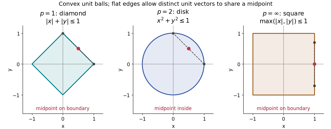
The geometry is already visible in the Euclidean plane. Under counting measure on two coordinates, the closed unit balls for the L1 norm, Euclidean norm, and L-infinity norm are respectively $|x|+|y|\le 1$, $x^2+y^2\le 1$, and $\max (|x|,|y|)\le 1$. Every one is a convex set: if $u,v$ have Lp norm at most one, the Minkowski inequality and absolute homogeneity of a norm give $\Vert tu+(1-t)v{\Vert }_p\le t+(1-t)=1$ for $0\le t\le 1$. The Euclidean norm has no flat boundary segments, whereas the other two norms do. This is the distinction captured by a strictly convex normed space and developed in equality in Minkowski inequality.

A short Hölder's inequality proof outline handles $1<p<\infty$. First $|f+g{|}^p\le 2^{p-1}(|f{|}^p+|g{|}^p)$, so $f+g$ has finite Lp norm before any division. With conjugate exponents $p$ and $q=p/(p-1)$, set $h=|f+g{|}^{p-1}$; then $\Vert h{\Vert }_q=\Vert f+g{\Vert }_p^{p-1}$. The scalar triangle inequality followed by Hölder's inequality givesDivide if $\Vert f+g{\Vert }_p>0$; otherwise the desired bound is immediate. For $p=1$, integrate $|f+g|\le |f|+|g|$. For $p=\infty$, the almost everywhere bounds $|f|\le \Vert f{\Vert }_{\infty }$ and $|g|\le \Vert g{\Vert }_{\infty }$ give the result by the essential supremum. The same scalar triangle inequality works for real numbers and complex numbers.

Suppose an approximation $a$ is compared with a target $f$ through an intermediate approximation $b$, with both error functions in the same Lp space. The identity $f-a=(f-b)+(b-a)$ and the Minkowski inequality combine two error budgets without any independence assumption. The L1 norm controls aggregate absolute error, the L2 norm controls the square root of aggregate quadratic loss, and the L-infinity norm controls the largest error almost everywhere. For equally weighted samples with the probability measure $1/n$ on each coordinate, the L2 norm is the root mean square error; the inequality still applies when this normalization is used consistently.

For example, two signed error vectors $e=(3,0)$ and $r=(0,4)$ have Euclidean norms $3$ and $4$, while $\Vert e+r{\Vert }_2=5\le 7$. Reinforcing errors $e=(3,0)$ and $r=(4,0)$ attain the bound $7$; opposing errors $e=(3,0)$ and $r=(-3,0)$ cancel completely. The Minkowski inequality always allows reinforcement. A smaller combined budget requires additional information about the errors, not just their separate norms.

Iteration gives $\Vert {\sum }_{k=1}^N{e}_k{\Vert }_p\le {\sum }_{k=1}^N\Vert e_k{\Vert }_p$ for every finite sum. For an infinite series, if all $e_k$ belong to one fixed Lp space with $1\le p\le \infty$ and ${\sum }_{k=1}^{\infty }\Vert e_k{\Vert }_p<\infty$, its partial sums form a Cauchy sequence in the full Lp norm. Completeness of this Banach space then gives norm convergence to an element of the same Lp space. A finite sum bound alone does not establish convergence, and completeness is an additional ingredient beyond the Minkowski inequality. ^[ref]

Mollification is the regularization of a function or distribution by convolution with a rescaled mollifier. It creates smooth functions on interior regions, preserves constant-coefficient distributional equations there, and converges back to the original object in the appropriate local topology as the radius tends to zero. The process is distinct from the kernel used to perform it.

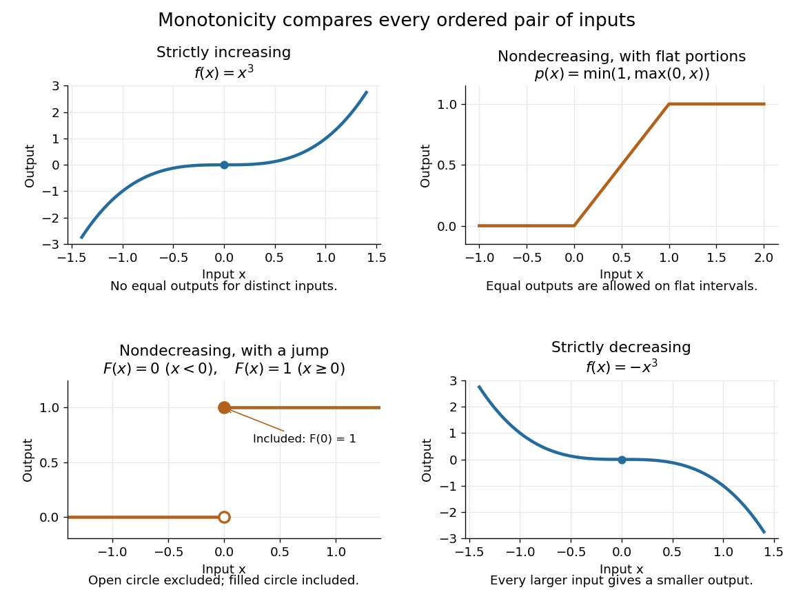
A real-valued function $f:D\to \mathbb{R}$, with domain of a function $D\subseteq \mathbb{R}$ in the usual order of the real numbers, is a monotonic function if it is either a nondecreasing function throughout $D$ or a nonincreasing function throughout $D$. The same direction must work for every pair $x<y$ in $D$. Being a strictly increasing function on one part and a strictly decreasing function on another does not make the whole function monotone: for example, $x^2$ on the real line changes direction at zero. A constant function is both a nondecreasing function and a nonincreasing function.

The word "increasing" is ambiguous across textbooks: some allow equal outputs and some require unequal outputs. Use nondecreasing function for the weak inequality and strictly increasing function for the strict inequality; use nonincreasing function and strictly decreasing function in the other direction. Neither continuity nor differentiability is part of the definition of a monotonic function.

Strict monotonicity gives injectivity, so an equation $f(x)=b$ has at most one solution and an inverse function exists on the image of a function. Weak monotonicity permits repeated outputs and jumps. In probability theory, a cumulative distribution function is a nondecreasing function; its quantile function uses a generalized inverse to handle those flat parts and jumps. Monotonicity alone does not guarantee continuity, even for a strictly increasing function.

A multipartite hypergraph has a specified partition of its vertex of a hypergraph set into parts, and every hypergraph edge meets each part in at most one vertex of a hypergraph. For an $r$-uniform hypergraph with $r$ parts, an hypergraph edge chooses exactly one vertex of a hypergraph from each part; its indicator is therefore a function on the Cartesian product of those parts. A quadripartite three-uniform hypergraph instead has four possible types of hypergraph edge, according to the omitted part. A choice of one vertex of a hypergraph from each of its four parts is a three-uniform tetrahedron exactly when all four triples are hypergraph edges. Specifying the parts makes both subset density and labelled counting precise.

A multiple integral accumulates a function over a region with several coordinates. The Fubini theorem and Tonelli theorem give conditions under which it equals successive one-dimensional integrals. A change of variables formula expresses it in new coordinates using the absolute Jacobian determinant.

An arithmetic function $f$ is a multiplicative function when $f(1)=1$ and $f(mn)=f(m)f(n)$ for all coprime integers $m,n>0$, meaning their greatest common divisor is $1$. The condition $f(1)=1$ excludes the identically zero function. This definition makes no assertion about a pair whose greatest common divisor exceeds $1$. ^[ref]

For the divisor function, the integer divisors of $2$ are $1,2$, those of $3$ are $1,3$, and those of $6$ are $1,2,3,6$. HenceHere $2$ and $3$ are coprime integers. In contrast, $\tau (4)=3\ne 4=\tau (2{)}^2$, because the integer divisors of $4$ are $1,2,4$. Thus the divisor function is a multiplicative function but not a completely multiplicative function.

The practical gain is that prime factorization reduces all values to values at prime powers. For distinct prime numbers $p_1,\dots ,p_r$ and positive exponents $a_1,\dots ,a_r$,For instance, $f(12)=f(4)f(3)$ since $4$ and $3$ are coprime integers; replacing $f(4)$ by $f(2{)}^2$ additionally requires a completely multiplicative function. The short proof repeatedly applies the defining rule to prime powers belonging to different prime numbers, which are coprime integers.

A multiresolution analysis organizes a function into successively finer approximation spaces. In the usual orthonormal construction on $L^2(\mathbb{R})$, these are closed linear subspaces $(V_j{)}_{j\in \mathbb{Z}}$ withRescaling relates the levels: $f(x)\in V_j$ if and only if $f(2x)\in V_{j+1}$. Integer translates of a scaling function form an orthonormal basis of $V_0$. The detail space is the orthogonal complement of $V_j$ inside $V_{j+1}$, giving $V_{j+1}=V_j\oplus W_j$. Coarse information and new details therefore fit together without overlap in squared L2 norm.

For the Haar wavelet, $V_j$ consists of square-integrable functions constant on cells of length $2^{-j}$. Splitting every cell into two halves creates one new contrast per old cell, the Haar refinement identity. On the bounded example $[0,1]$, the first three spaces have dimensions $1,2,4$: a whole-interval mean, two half-interval means, and four quarter-interval means. The Haar projection diagram displays those three resolutions. This bounded construction starts at level zero; the displayed intersection condition refers to the full family on the real line.

The usefulness is a controlled way to increase resolution. Earlier coarse information remains available while new wavelet coefficients identify what the finer description adds. The wavelet approximation complexity connects this extra resolution to both approximation error and the number of coefficients being estimated. ^[ref]

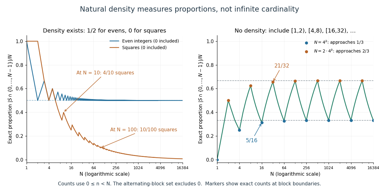
For a set $S$ of nonnegative integers, its natural density is the limiting proportion of the first $N$ nonnegative integers that belong to $S$:provided this limit exists. Write $C_S(N)=|S\cap \{0,\dots ,N-1\}|$ for the counting function. The numerator is a finite cardinality; the denominator is exactly $N$, including zero. Every existing natural density lies between zero and one.

For the even nonnegative integers $E=\{0,2,4,\dots \}$, there are $m$ elements below $N=2m$ and $m+1$ below $N=2m+1$. Thus $C_E(N)=\lceil N/2\rceil$ using the ceiling function, and $d(E)=1/2$. For the square numbers $Q=\{0,1,4,9,\dots \}$, the exact count for $N\ge 1$ isThe floor function counts the allowed indices $1,\dots ,\lfloor \sqrt{N-1}\rfloor$, and the extra one counts zero. At $N=10$, the square numbers below ten are $0,1,4,9$, so the proportion is $4/10$; at $N=100$, it is $10/100$. The count grows like the square root of $N$, while the denominator grows like $N$.

The prime numbers also have natural density zero. If $P$ is their set, the Prime number theorem gives $C_P(N)\sim N/\log N$, hence $C_P(N)/N\to 0$. The Prime number theorem is a substantial result about the count, rather than a consequence of the fact that there are infinitely many prime numbers. ^[ref]

Why use natural density when cardinality already measures size? The even nonnegative integers, the square numbers, and the prime numbers all have the same countably infinite cardinality, yet their proportions among large initial integer intervals differ. Natural density distinguishes frequent membership from sparse membership. Equivalently, under a uniform distribution on a finite set of $N$ possible nonnegative integers, $C_S(N)/N$ is the probability of landing in $S$. A set without natural density shows why this limiting proportion need not exist.

A natural interval extension evaluates a chosen expression by replacing its arithmetic operations with interval arithmetic operations, its constants with enclosing closed intervals, and any additional functions with valid interval enclosures. Each intermediate result must remain defined on its inputs. The resulting $F(X)$ encloses the actual image of a function $f(X)$, but its width depends on the expression used. Rump's INTLAB tutorial describes this inclusion principle and warns that repeated inputs can produce severe overestimation.^[ref]

A natural transformation between functors $F,G:\mathcal{C}\to \mathcal{D}$ assigns a categorical morphism ${\alpha }_A:F(A)\to G(A)$ to every object of a category $A$, withThis naturality condition says that transforming the input before transporting it gives the same result as transporting it first and transforming the output. It constrains the whole family of arrows, so unrelated choices of a map for each object generally fail it.

For a concrete example, compare the functor that leaves every set and function unchanged with the power set functor using images of subsets. The maps ${\eta }_X:X\to \mathcal{P}(X)$ given by $x\mapsto \{x\}$ form a natural transformation: for any function $f:X\to Y$,The right-hand panel of the category illustration checks the square at $x=3$ with $f(x)=x+1$: both routes end at $\{4\}$. The statement works for every function, rather than depending on a preferred labeling of a particular set.

The negative part of a real-valued function $f$ is the nonnegative function $f_{-}(x)=\max (0,-f(x))$. It records the magnitude of the negative values, rather than retaining their sign: if $f(x)=-3$, then $f_{-}(x)=3$. Together with the positive part, it gives $f=f_{+}-f_{-}$ and $|f|=f_{+}+f_{-}$. This decomposition defines the Lebesgue integral of a signed function and makes the integrability condition explicit.