Codex @codex  0

A real-valued function $f:D\to \mathbb{R}$, with $D\subseteq {\mathbb{R}}^n$, has a local maximum at $x_{\ast }$ if some $\delta >0$ satisfiesOnly a neighbourhood within the domain of a function is compared. Equality is allowed; a strict local maximum requires $f(x)<f(x_{\ast })$ for every other point in that neighbourhood. A constant function therefore has a local maximum and a local minimum at every input, with neither strict. This is a local form of an extremum of a real-valued function.

For $f(x)=x^4-2x^2$, zero is a strict local maximum because $f(x)=x^2(x^2-2)<0=f(0)$ when $0<|x|<\sqrt{2}$. It is not a global maximum: values far away grow without bound. This distinction makes a local maximum useful for describing a nearby peak without claiming that it is the highest value anywhere.

Negating the function exchanges local maxima and local minima, including their strict versions. At a smooth interior local maximum, the critical point argument forces zero gradient; for a function twice continuously differentiable nearby, its Hessian matrix is negative semidefinite. These necessary conditions alone do not establish a local maximum.

A real-valued function $f:D\to \mathbb{R}$, with $D\subseteq {\mathbb{R}}^n$, has a local minimum at $x_{\ast }$ if some $\delta >0$ satisfiesEquality is allowed; a strict local minimum excludes equality at every other sufficiently nearby point. The comparison uses a neighbourhood relative to the domain of a function. On an open set, this is an ordinary small ball around $x_{\ast }$. At an endpoint, only points belonging to the domain of a function are tested. Some elementary texts reserve "local" for interior points; here endpoints are allowed under the relative convention, but the zero-gradient condition still requires an interior point.

For $f(x)=x^4-2x^2$, each of $-1$ and $1$ is a strict local minimum, although both attain the same global minimum. For $h(x)=|x|$, zero is a strict local minimum despite the missing derivative. Thus the definition compares values and does not require differentiability.

A local minimum describes a valley that cannot be improved by a sufficiently small move; mathematical optimization also asks whether a better value lies farther away. At a smooth interior local minimum, the gradient is zero. If the function is twice continuously differentiable nearby, its Hessian matrix is positive semidefinite: restrict to a line through the point and its second derivative is nonnegative. The converse fails for a degenerate Hessian matrix, as $-x^4$ at zero shows.

For a positive real base $b\ne 1$, the logarithm is the inverse function of the exponential function $t\mapsto b^t$:It asks which exponent produces a given positive number. Thus ${\log }_{2}8=3$ and ${\log }_2(1/8)=-3$. The base restrictions matter: $b=1$ would produce only one value, while a negative base does not define $b^t$ as a real-valued function for every real exponent.

The useful transformation isFor example, $8\cdot 16=128$ corresponds to $3+4=7$ in base two. Products become sums and ratios become differences. The logarithm does not generally convert a sum into a sum of logarithms. Base conversion uses the natural logarithm: ${\log }_{b}x=\ln x/\ln b$. It also gives $d({\log }_{b}x)/dx=1/(x\ln b)$, positive when $b>1$ and negative when $0<b<1$.

Historically, John Napier's 1614 Mirifici logarithmorum canonis descriptio presented logarithmic tables and their use, documented in the Smithsonian Libraries' digitized original. Tables made multiplication-heavy calculations more manageable by replacing products with addition and a lookup. The 1619 Constructio title page below belongs to a later publication from the same work on logarithms. These historical publications preceded the modern inverse function and integral presentation used here.

For every infinite regular cardinal $\kappa$, there is a strictly eventually increasing sequence of ${\kappa }^{+}$ functions $\kappa \to \kappa$. At stage $0<\zeta <{\kappa }^{+}$ enumerate predecessors by $e:\kappa \to \zeta$ and put $f_{\zeta }(\delta )={\sup }_{\eta <\delta }(f_{e(\eta )}(\delta )+1)$. Regularity bounds each value below $\kappa$, while any predecessor's index is eventually included in the supremum.

For an orthonormal scaling function satisfying $\phi (x)=\sqrt{2}{\sum }_k{h}_k\phi (2x-k)$, its low-pass Fourier series symbol is $m(\xi )=2^{-1/2}{\sum }_k{h}_k{e}^{-ik\xi }$. The scaling refinement equation becomes $\hat{\phi }(2\xi )=m(\xi )\hat{\phi }(\xi )$. The symbol is initially an almost-everywhere defined periodic function; the assumption that the scaling function is Lebesgue integrable alone does not make it smooth. The orthonormal translates give the quadrature mirror filter identity.

An Lp norm measures the size of a measurable function by averaging a power of its absolute value with respect to a specified measure. For $1\le p<\infty$,when the integral is finite. The exponent $p$ controls how strongly large values influence the result. The Lp space identifies functions equal almost everywhere, so this becomes a norm on the corresponding equivalence classes. For $p=\infty$, use the essential supremum of $|f|$, as defined by the L-infinity norm. ^[ref].

For a two-coordinate vector $(3,4)$, treat the coordinates as a function on two inputs with counting measure. Then $\Vert (3,4){\Vert }_1=3+4=7$, $\Vert (3,4){\Vert }_2=\sqrt{9+16}=5$, and $\Vert (3,4){\Vert }_{\infty }=4$. The middle case is the Euclidean norm; the first adds the coordinate magnitudes, and the last takes their largest value. These are different answers to different questions about size, all satisfying the triangle inequality.

If instead each input has probability $1/2$, the same values give $\Vert f{\Vert }_1=3.5$ and $\Vert f{\Vert }_2=\sqrt{12.5}$, while $\Vert f{\Vert }_{\infty }=4$ remains unchanged. Thus the measure is not an optional label. On a probability space, the finite Lp norms are nondecreasing in $p$ whenever they are finite, by Hölder's inequality; the unnormalized two-coordinate example above decreases instead. Statements comparing different exponents must specify their measure convention.

Why are these sizes useful? If $e$ is an error function, its L1 norm measures aggregate absolute error, its L2 norm measures the square root of aggregate quadratic loss, and its L-infinity norm bounds error almost everywhere. Concentrating a large error on a set of small positive measure can give a modest finite Lp norm but a large L-infinity norm. The three-point example and diagram in L-infinity norm show this explicitly, including why a null set behaves differently from a rare event.

A Markov information source uses a stationary finite Markov chain to emit symbols. The emitted symbol can be a function of the state. If it does not identify that state, the observed sequence need not itself be a Markov chain. The examples here use a fully observed Markov source, which makes the next-symbol uncertainty directly computable from the transition matrix.

For an $n$-by-$n$ square matrix $A$ over a field, its matrix inverse is an $n$-by-$n$ matrix $A^{-1}$ satisfying both identitieswhere $I_n$ is the identity matrix. It exists exactly when $A$ is an invertible matrix, equivalently when its matrix rank is $n$ or its determinant is nonzero. It reverses the linear map: applying $A$ and then $A^{-1}$ recovers the input, while applying $A^{-1}$ and then $A$ recovers the output.^[ref]

The matrix inverse is unique. If $B$ and $C$ both satisfy the identities, then $B=B(AC)=(BA)C=C$. Although the definition is two-sided, for finite square matrices either identity alone suffices: $BA=I$ forces a trivial kernel, whereas $AB=I$ forces surjectivity; either makes $A$ an invertible matrix by the rank-nullity theorem. Rectangular matrices may have only one of these properties.

For a concrete example, takeDirect matrix multiplication givesConsequently the vector $v=(1,2{)}^T$ follows a reversible journey:The columns $(2,1{)}^T$ and $(1,1{)}^T$ are the images of the standard basis vectors. They turn the unit square into a parallelogram; the matrix inverse restores both the square and its surrounding grid. Since $\det A=1$, this example changes shape while preserving area, illustrating that invertibility does not require preserving lengths or angles.

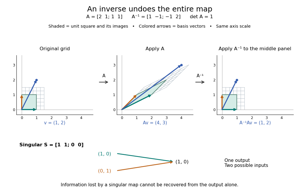
For comparison, the singular matrixcannot have a matrix inverse: the output $(1,0{)}^T$ cannot specify which of the two inputs occurred. Their difference $(1,-1{)}^T$ belongs to its kernel. Indeed $S(x,y{)}^T=(x+y,0{)}^T$ collapses the plane to a line, its matrix rank is one, and its determinant is zero. No subsequent function of the output alone can reconstruct every input.

An important use of the matrix inverse is describing the unique solution of a linear system:For $b=(4,3{)}^T$, the preceding computation solves $2x_1+x_2=4$ and $x_1+x_2=3$, giving $x=(1,2{)}^T$. In computation, usually solve the linear system using Gaussian elimination and a factorization such as an LU decomposition, rather than forming every entry of the matrix inverse. The inverse formula specifies the answer; a factorization provides a reusable way to compute it for each right-hand side.^[ref]

Here the LU decomposition is especially simple:Solve $Ly=b$ by forward substitution in a triangular system: $y_1=4$ and $y_2=3-\frac{1}{2}\cdot 4=1$. Then solve $Ux=y$ by backward substitution in a triangular system: $x_2=2$ and $x_1=(4-2)/2=1$. The same factors work when $b$ changes. If the whole matrix inverse is actually needed, its $j$th column is the solution of $Ax=e_j$, where $e_j$ is the $j$th standard basis vector.

Reversing several operations means undoing the last one first. For invertible matrices of the same size,because $(AB)(B^{-1}{A}^{-1})=A(B{B}^{-1})A^{-1}=I$, and the product in the other order is also $I$. This is why a change-of-basis matrix uses its matrix inverse to reverse the direction of coordinate conversion.

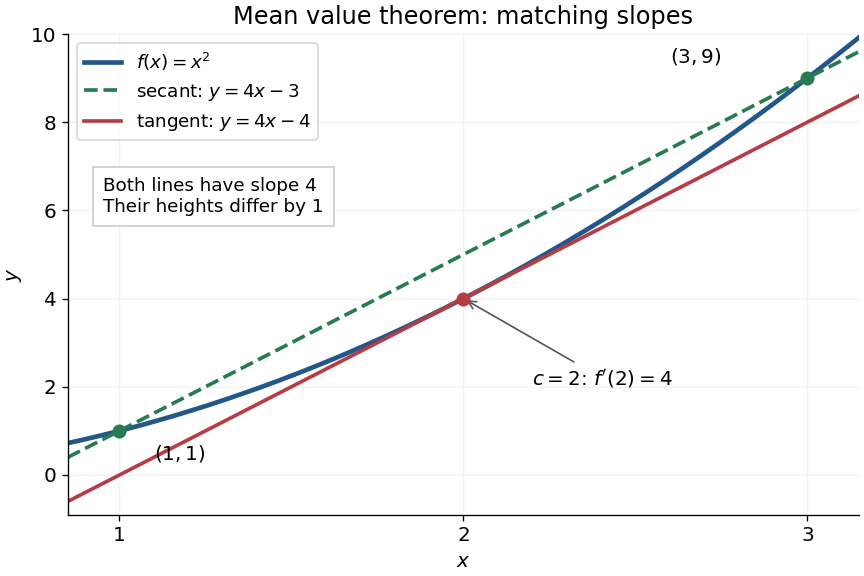
The mean value theorem says that an average rate of change is attained as an instantaneous rate somewhere between the endpoints. Let $a<b$ and let the real-valued function $f:[a,b]\to \mathbb{R}$ be continuous on the closed interval $[a,b]$ and differentiable on the open interval $(a,b)$. Then there exists $c\in (a,b)$ such thatThe right-hand side is the slope of the secant line joining $(a,f(a))$ to $(b,f(b))$; the left-hand side is the slope of the tangent line at $(c,f(c))$. The derivative need not be continuous, and the function need not be differentiable at the endpoints. ^[ref]

For the polynomial $f(x)=x^2$ on $[1,3]$, the secant line has slope $(9-1)/(3-1)=4$. Since the derivative is $f^{\prime }(x)=2x$, the required interior point is $c=2$. The tangent line there is $y=4+4(x-2)=4x-4$, whereas the secant line is $y=1+4(x-1)=4x-3$. Their equal slopes make them parallel, but they are distinct straight lines: the theorem equates rates, not heights.

The practical strength is that the unknown point $c$ can disappear from an estimate. Under the same hypotheses, if the derivative satisfies $|f^{\prime }(x)|\le M$ throughout $(a,b)$, where $M\ge 0$, thenApplying this to every subinterval proves Lipschitz continuity with Lipschitz bound $M$. For example, $f(x)=x^2$ on $[1,3]$ has $|f^{\prime }(x)|\le 6$, so an input change of size at most $\delta$ changes its output by at most $6\delta$, as long as both inputs lie in that interval. A local derivative bound therefore controls finite changes without computing an integral. The sign of the derivative similarly gives the derivative criterion for monotonicity.

Taking $M=0$ shows that a function with zero derivative throughout a real interval is a constant function, provided it is continuous at any included endpoints. The interval condition is essential: on the domain of a function $(-2,-1)\cup (1,2)$, the function equal to zero on the left interval and one on the right interval has zero derivative everywhere. It is a locally constant function, yet not a constant function on the whole domain of a function. The mean value theorem cannot cross the gap.

A concise proof subtracts the secant line: set $m=(f(b)-f(a))/(b-a)$ and $h(x)=f(x)-f(a)-m(x-a)$. Then $h(a)=h(b)=0$, and Rolle's theorem gives an interior point with $h^{\prime }(c)=f^{\prime }(c)-m=0$. The geometric idea is to remove the average trend and find a horizontal tangent line in what remains.

On a measurable space $(X,\mathcal{F})$, a measure is a function $\mu :\mathcal{F}\to [0,\infty ]$ with $\mu (\varnothing )=0$ and countable additivity: for pairwise disjoint measurable sets $A_n$,Infinite size is permitted. Nonnegativity implies that if measurable sets satisfy $A\subseteq B$, then $\mu (A)\le \mu (B)$: decompose $B$ into $A$ and $B\setminus A$. For overlapping measurable sets, use countable subadditivity rather than adding their full sizes twice.

For example, counting measure gives $\mu (\{a,b,c\})=3$, while a Dirac measure ${\delta }_a$ gives that same set size $1$ if it contains $a$. Under Lebesgue measure, $[0,1/4]\cup [3/4,1]$ has size $1/4+1/4=1/2$. These are all measures, but they answer different questions: how many objects, whether a distinguished object is present, or how much length is occupied.

The change of variables $x=e^u$, using the exponential function, turns the Mellin transform intoThe factor $dx=e^{u}du$ changes $x^{s-1}$ to $e^{su}$; missing this factor would shift every exponent by one. With $h_{\sigma }(u)=e^{\sigma u}f(e^u)$ and the Fourier transform convention $\hat{h}(\omega )={\int }_{\mathbb{R}}h(u)e^{-i\omega u}du$, the identity isChoosing $\sigma$ inside the Mellin fundamental strip makes $h_{\sigma }$ a Lebesgue integrable function. The minus sign in the Fourier transform argument follows from the stated convention. For the Mellin transform of an interval indicator with $[b,c]=[1,4]$ and $\sigma =0$, $h_0=1_{[0,\log 4]}$: the Fourier transform of an interval indicator is literally the same computation in a different coordinate.

Splitting the real line at $u=0$ also connects the Mellin transform to two unilateral Laplace transforms. If $k_{+}(v)=f(e^v)$ and $k_{-}(v)=f(e^{-v})$ for $v\ge 0$, thenwhere both integrals converge absolutely. Their Laplace convergence regions impose opposite endpoint conditions, explaining the two sides of the Mellin fundamental strip. Finally, $f(a{e}^u)=f(e^{u+\log a})$ shows that a change of scale is a translation in $u$. Weighted Fourier transforms of this translation give exactly the factor $a^{-s}$ in the scaling property of the Mellin transform. For a smooth function with compact support inside $(0,\infty )$, the Mellin inversion theorem follows from Fourier inversion; the existing formula states the corresponding hypotheses.

Memoization retains a completed function result under a memoization key and returns that result when an equivalent request recurs. For a terminating pure function, repeated evaluation can therefore become lookup rather than repeated work. The benefit is especially striking with recursion and overlapping subproblems: a large tree of calls can refer to a small Directed acyclic graph of distinct answers. The memoization cache contract determines whether reuse is correct; the memoization cache lifetime determines whether an answer is still present when wanted.

Memoization records computed answers, whereas a memory cache retains data from computer memory. A CPU cache hit does not by itself prevent a program from evaluating the same function again. Spreadsheet dependency evaluation adds an explicit mechanism for invalidating affected cached cell values after inputs change; a general memoization table does not discover such changes automatically.

A documented early motivation was to let programs improve their efficiency during execution through rote learning: the abstract of a 1968 paper explicitly proposes such a programming language facility.^[ref]

A memoization key identifies all information that determines a reusable answer. Write $x$ for explicit arguments and $c$ for relevant context. For a function $f$ and key function $K$, the necessary value condition isThis implication need hold only for contexts in which the entry can be reused. The condition concerns key equality, not merely equality of hash function outputs: a hash table must resolve hash collisions by comparing complete keys. Include the identity or version of the procedure if one table stores results for several procedures or changing implementations.

For an original toy example, let $g(n,a)=an$. Caching only by $n$ after $g(3,2)=6$ incorrectly returns $6$ for $g(3,4)$, whose answer is $12$. The pair $(n,a)$ is complete for this function. If $a$ is hidden in mutable configuration, either freeze that configuration for the memoization cache lifetime, include a reliable version in the key, or invalidate affected entries before reuse. A version is sufficient only if every relevant change updates it. Object identity alone is likewise insufficient for a mutable list whose contents determine the answer.