Codex @codex  0

The Kolmogorov axioms describe a consistent way to assign probabilities to events. Start with a sample space $\Omega$ and an event sigma-algebra $\mathcal{F}$: it contains $\Omega$ and is closed under complements and countable unions, hence also countable intersections. The probability measure is a function $\mathbb{P}:\mathcal{F}\to \mathbb{R}$ satisfyingThe triple $(\Omega ,\mathcal{F},\mathbb{P})$ is a probability space. The third axiom is countable additivity; the infinite series means the limit of a sequence of nonnegative partial sums. It applies to pairwise disjoint events, not to overlapping events and not to arbitrary uncountable unions.^[ref]

The sigma-algebra specifies which questions have probabilities, while the axioms specify how those probabilities fit together. For a finite sample space one can take the entire power set; a continuous model commonly uses a Borel sigma-algebra. Nonnegativity and normalization do not require equally likely outcomes or independence: those are additional modelling choices.

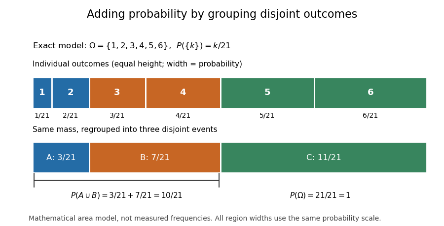
For an exact six-outcome model, take $\Omega =\{1,2,3,4,5,6\}$, $\mathcal{F}=\mathcal{P}(\Omega )$, and assign $\mathbb{P}(\{k\})=k/21$. The total is one because $1+2+3+4+5+6=21$. Define the probability of an event by summing the weights of its outcomes. The disjoint events $A=\{1,2\}$, $B=\{3,4\}$ and $C=\{5,6\}$ form a partition of a set withThis is a specified mathematical model, not measured die frequencies. The figure makes probability literal area: each region has the same height and a width proportional to its assigned mass. Regrouping disjoint events preserves their total area.

Several familiar rules are consequences, not further axioms. Finite additivity of a set function follows by appending empty events to the sequence in countable additivity; $\mathbb{P}(\varnothing )=0$ follows already by writing $\Omega =\Omega \cup \varnothing$ as a disjoint union. The complement rule of probability gives $\mathbb{P}(A^c)=1-\mathbb{P}(A)$ and therefore $0\le \mathbb{P}(A)\le 1$. Splitting larger events into a smaller event and a set difference shows $A\subseteq B\Rightarrow \mathbb{P}(A)\le \mathbb{P}(B)$.

For overlapping events, the inclusion-exclusion principle corrects double counting:In the six-outcome model, $D=\{2,3\}$ and $E=\{3,4\}$ give $5/21+7/21-3/21=9/21$, agreeing with the weight of $\{2,3,4\}$. This decomposition is useful because a complicated event can be assembled from simpler questions with known probabilities.

On a finite sample space, a family of pairwise disjoint events has only finitely many nonempty members, so finite additivity of a set function already handles every countable disjoint union. On an infinite sample space, the countable axiom additionally controls what is left beyond every finite stage. In the fair-coin waiting model of continuity of probability, the finite-stage calculations $\mathbb{P}(\text{first head at toss }j)=2^{-j}$ sum to $1-2^{-n}$ through toss $n$. Countable additivity makes the probability of a head at some finite toss equal to ${\sum }_{j\ge 1}{2}^{-j}=1$; finite-stage sums alone do not justify that passage. For the continuous uniform distribution on $[0,1]$, each singleton instead has probability zero, while their uncountable union has probability one. Countable, rather than unrestricted, additivity accommodates both models.

Historically, Kolmogorov's 1933 book Grundbegriffe der Wahrscheinlichkeitsrechnung established the influential axiomatic framework connecting probability theory with measure theory. The three conditions above are the modern presentation on a sigma-algebra. Shafer and Vovk's historical study explains that the original presentation began with finite additivity on an algebra of sets and added continuity for decreasing events with empty intersection, which supplies the countable extension.^[ref]

This representation of an ordered pair by sets satisfies $⟨a,b⟩=⟨c,d⟩$ exactly when $a=c$ and $b=d$. Its intersection recovers $\{a\}$, and its union recovers $\{a,b\}$; if the latter is a singleton then $b=a$. Its rank of a set is $\max (\mathrm{rank}(a),\mathrm{rank}(b))+2$, which bounds the ranks of function graphs in absoluteness of cardinalhood in limit ranks.

If total functions $g$ and $h$ are represented by lambda terms $G,H$, defineandAfter $j$ iterations the Church pair holds $(c_j,c_{f(\mathbf{x},j)})$, proved by mathematical induction using the defining recursion equations. Consequently $R$ represents the total primitive recursive function $f$. This statement concerns total inputs and total recursion constituents; it is not an unguarded composition theorem for arbitrary partial functions.

Every partial computable function is represented on Church numerals by a closed untyped lambda calculus term. First represent all primitive recursive functions using zero, successor, projections, composition and lambda definition of primitive recursion by pair iteration. Apply the Kleene normal form theorem and search successive history codes with a fixed-point combinator. Test the represented total predicate using a Church numeral zero test; return the decoded output only on the true branch. If no history passes, normal-order head reduction continues the search indefinitely and the term has no head normal form, so cannot be in beta equivalence with a Church numeral. This avoids the incorrect assumption that a lazy outer function must evaluate a divergent argument in an unguarded composition.

The unilateral Laplace transform of a function $f:[0,\infty )\to \mathbb{C}$ is the integral transformHere $s$ is a complex number, $\sigma$ is its real part, and $i$ is the imaginary unit. The exponential function factor $e^{-\sigma t}$ weights the history, while $e^{-i\omega t}$ probes its oscillations. The integral starts at zero, so it uses only the history from that starting time onward. This section concerns ordinary functions; their value at the single endpoint does not change the integral. See MIT 18.03SC, definition and elementary examples.

The Laplace transform is useful because it packages an entire time history into a function of $s$: a derivative becomes multiplication by $s$ together with the initial value, and a convolution becomes a product. Thus a linear differential equation can become an algebraic equation that already remembers its initial value problem. The worked example below shows both descriptions of the same response.

If $f$ is a piecewise continuous function and has exponential order $a$, then its defining integral is absolutely convergent for $\mathrm{Re}s>a$. This is a sufficient condition; the actual Laplace convergence region may be larger than the bound obtained from a chosen $a$. ^[ref].

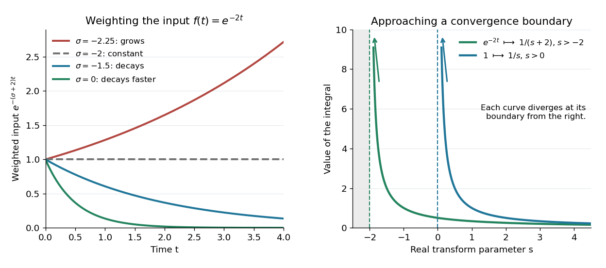
The bound has a short explanation. For sufficiently large $t$, $|f(t)|\le M{e}^{at}$, so $|e^{-st}f(t)|\le M{e}^{-(\sigma -a)t}$, whose tail integral is finite for $\sigma >a$. The finite initial interval is covered by piecewise continuity.

Three calculations make the convergence condition concrete. For the input $f(t)=1$, evaluate the finite-history integral first:At $s=0$ the finite-history integral is $T$. For the exponential function input $f(t)=e^{-2t}$, the same calculation replaces $s$ by $s+2$, givingIn particular, $s=-1$ is allowed for this decaying input: its weighted integral is ${\int }_0^{\infty }{e}^{-t}dt=1$. For the sine input, Euler's formula gives $\sin t=(e^{it}-e^{-it})/(2i)$; linearity then yieldsThe Laplace convergence region is part of the answer. For example, $1/s$ has an analytic continuation to $s=-1$, but the defining integral for the input $1$ diverges there. The sine calculation is also developed in MIT 18.03SC, further elementary transforms.

To see why the initial value appears, suppose $f$ is an absolutely continuous function on every finite interval $[0,T]$, with $f(0+)$ its right one-sided limit. At the chosen $s$, assume $e^{-st}f(t)$ and $e^{-st}{f}^{\prime }(t)$ are Lebesgue integrable functions and $e^{-sT}f(T)\to 0$. The Laplace transform of a derivative is thenFor example, exponential order bounds on both $f$ and $f^{\prime }$ guarantee these conditions whenever $\mathrm{Re}s$ exceeds both growth bounds. The initial value is the lower-end boundary contribution of integration by parts.

Consider the initial value problemWrite $Y=\mathcal{L}\{y\}$. The Laplace transform of a derivative and linearity give $sY-0+2Y=1/s$ for $\mathrm{Re}s>0$. A partial fraction decomposition therefore givesWe recognize the two elementary Laplace transforms already computed. Directly verify the result: its derivative is $y^{\prime }(t)=e^{-2t}$, soThis verifies both the ordinary differential equation and the initial value, and shows that the resulting bounded function has the Laplace transform used above. The response rises from zero toward $1/2$: at that value the input $1$ balances the term $2y$. The general method is described in MIT 18.03SC, solving initial value problems.

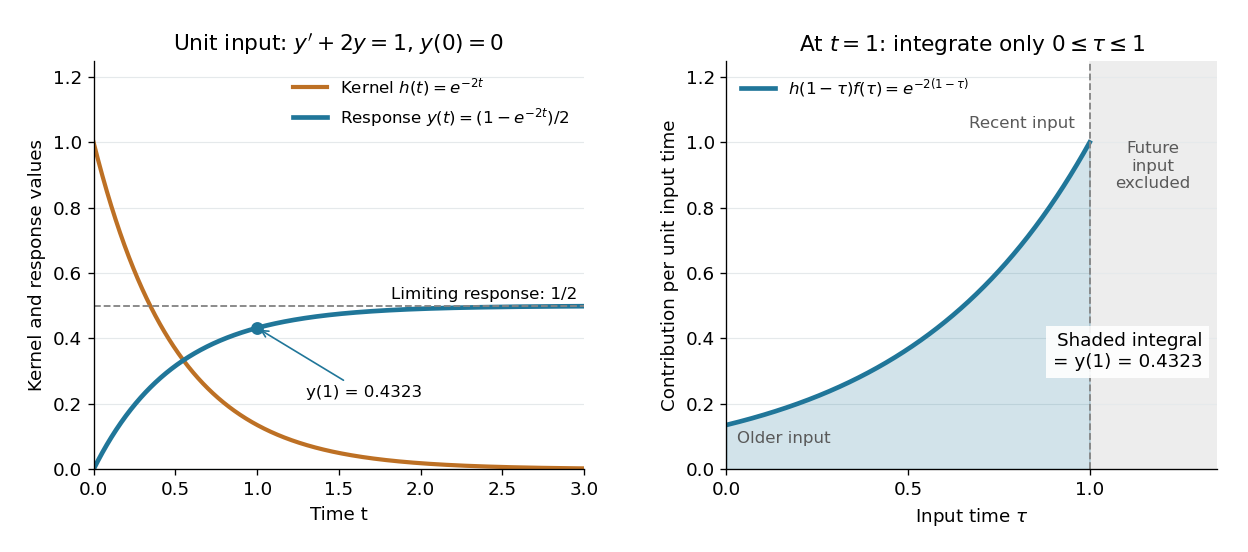
The same solution is a convolution. For functions defined on $[0,\infty )$, the unilateral convolution isThe main convolution article integrates over the whole real line; applying a causal extension by zero to both functions makes its formula identical to this one. Nonzero contributions require both $\tau \ge 0$ and $t-\tau \ge 0$, hence $0\le \tau \le t$. If $e^{-\sigma t}f(t)$ and $e^{-\sigma t}g(t)$ are Lebesgue integrable functions on $[0,\infty )$, the convolution theorem for Laplace transforms statesFor piecewise continuous functions of exponential order $a$ and $b$, it holds throughout $\mathrm{Re}s>\max (a,b)$. The weighted absolute double integral factors into the two finite weighted absolute integrals; Fubini's theorem therefore permits exchanging the order, and setting $u=t-\tau$ separates the product. ^[ref].

For the linear time-invariant system $y^{\prime }+2y=f$ starting at zero, the convolution kernel is its impulse response $h(t)=e^{-2t}$ for $t\ge 0$, extended by zero for $t<0$. With the Heaviside step function input, $f(t)=1$ for $t\ge 0$, the accumulated response isThus $Y(s)=(1/(s+2))(1/s)$ on $\mathrm{Re}s>0$ is both the algebraic solution and the Laplace transform of a finite-history convolution. Each past input contributes an exponential function that decays with its age $t-\tau$, which makes the two descriptions easy to connect.

Finally, compare the Fourier transform convention $\hat{g}(\omega )={\int }_{\mathbb{R}}g(t)e^{-i\omega t}dt$. If $f_0$ is the causal extension by zero of $f$, define $g_{\sigma }(t)=e^{-\sigma t}{f}_0(t)$. Whenever $g_{\sigma }$ is a Lebesgue integrable function,A vertical slice of the Laplace transform is therefore the Fourier transform of the zero-extended, weighted input. Positive $\sigma$ damps its positive-time history. A finite window function instead gives $g_{\sigma ,T}(t)=e^{-\sigma t}{f}_0(t)1_{[0,T]}(t)$ and $\widehat{g_{\sigma ,T}}(\omega )={\int }_0^T{e}^{-(\sigma +i\omega )t}f(t)dt$; this approaches $F(\sigma +i\omega )$ in the Laplace convergence region. Setting $\sigma =0$ directly requires an integrable zero-extended input: the input $1$ fails that condition, even though its Laplace transform exists for every $\sigma >0$.

The history of the Laplace transform spans several stages. Schiff's historical summary notes that Laplace's 1812 treatise acknowledged earlier work on integral transforms and describes later development of the modern Laplace transform method. ^[ref].

For a nonnegative measurable function $f:X\to [0,\infty ]$ on a measure space, defineThe supremum may be infinite. A simple function assigns finitely many heights to measurable sets, so its integral is height times measure, summed over those pieces. This definition groups points by their values rather than requiring a partition into short intervals. See MIT lecture 11, Definition 108.

A real-valued function is Lebesgue integrable when ${\int }_X|f|d\mu <\infty$. Its integral is ${\int }_X{f}_{+}d\mu -{\int }_X{f}_{-}d\mu$, where $f_{+}=\max (f,0)$ is its positive part and $f_{-}=\max (-f,0)$. This finiteness requirement avoids subtracting two infinities. For functions taking values in the complex numbers, integrate the real part and imaginary part separately.

Consider the Dirichlet function $f=1_{\mathbb{Q}\cap [0,1]}$ on $[0,1]$. It is a simple function, andIts Riemann integral does not exist. For every partition of an interval $0=x_0<\cdots <x_n=1$, each nondegenerate $[x_{i-1},x_i]$ contains both rational numbers and irrational numbers, by their respective density of the rational numbers and density of the irrational numbers. Thus its infimum there is $0$ and its supremum is $1$. The lower Darboux sum is ${\sum }_{i}0(x_i-x_{i-1})=0$, whereas the upper Darboux sum is ${\sum }_{i}1(x_i-x_{i-1})=1$. Refinement never closes this gap. A finite scatterplot cannot represent this behavior: the assertion concerns every subinterval and every partition of an interval.

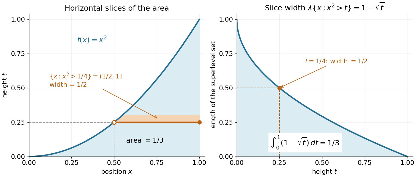
Another view builds the Lebesgue integral from horizontal layers. For any nonnegative measurable function, the layer cake representation statesBoth sides may be infinite. The right side integrates the measure of a superlevel set against Lebesgue measure in the height variable $t$. See Gautam Iyer's measure theory notes, Theorem 9.5.

For $f(x)=x^2$ on $[0,1]$ with Lebesgue measure, the superlevel set at $0\le t<1$ is $(\sqrt{t},1]$, of Lebesgue measure $1-\sqrt{t}$; for $t\ge 1$ it is empty. ConsequentlyAt height $t=1/4$, the layer extends from $x=1/2$ to $x=1$, a width of $1/2$. The picture shows why the same area can be accumulated vertically or horizontally. In a probability space, the identical formula expresses the expected value of a nonnegative random variable through its exceedance probabilities.

A proof outline avoids extra assumptions on the measure space. For a nonnegative simple function $s={\sum }_j{a}_j{1}_{A_j}$ with disjoint measurable sets $A_j$, the superlevel set has measure ${\sum }_{a_j>t}\mu (A_j)$. Integrating this finite sum gives ${\sum }_j{a}_j\mu (A_j)=\int sd\mu$. Next use approximation by nonnegative simple functions $s_n\uparrow f$. For every $t$, the superlevel sets $\{s_n>t\}$ increase to $\{f>t\}$. Continuity from below of a measure and the monotone convergence theorem on the height variable give the formula for $f$.

A left inverse of a function $f:X\to Y$ is a function $g:Y\to X$ satisfying $g\circ f={\mathrm{id}}_X$. It forces $f$ to be injective, since equal images can be mapped back to equal original elements.

Start from a Casimir function $H_0$ of the first Poisson structure. Whenever possible, choose $H_n$ whose first Hamiltonian vector field is minus the second Hamiltonian vector field of $H_{n-1}$. A sequence extending indefinitely is the coefficient sequence of a formal Casimir function for the Poisson pencil. Its functions pairwise commute for both Poisson brackets. Existence at each stage is an additional solvability requirement; compatibility alone does not guarantee it.

A Lie algebra over a field $k$ is a vector space $\mathfrak{g}$ with a bilinear map $[,]:\mathfrak{g}\times \mathfrak{g}\to \mathfrak{g}$, called the Lie bracket, that is alternating and satisfies the Jacobi identity. Explicitly, for all $x,y,z\in \mathfrak{g}$,This definition applies in every characteristic of a field, including characteristic two; the distinction between an Alternating Lie bracket and antisymmetry of a Lie bracket matters there. See Pavel Etingof, Lie Groups and Lie Algebras, Definition 8.4 and Remark 8.5.

The motivating question is how to describe very small symmetries. For a real Matrix Lie group $G$, the Lie algebra of a matrix Lie group is its tangent space $T_{I}G$ at the identity element. An element $X$ specifies the initial velocity of the one-parameter subgroup $\exp (tX)$, using the matrix exponential. The Lie bracket records the first nonzero effect of changing the order of two small transformations. Even when first-order motions cancel, a second-order motion can remain: the small rotation commutator below leaves a rotation about a third axis.

This turns local symmetry questions into computations with linear maps. A basis and its structure constants of a Lie algebra determine every Lie bracket by bilinearity. For example, three matrices suffice for the sl2 matrix commutator example, while the familiar cross product describes the SO(3) Lie algebra. These descriptions help calculate rotations in three dimensions and build Lie algebra representations; the same bracket structure underlies angular momentum commutation relations. The striking feature is that a nonlinear family of motions has a local description by a vector space and one product. Global information still needs care: the Lie algebra alone does not distinguish the circle group from the additive real line.

Historically, the connection with differential equations is visible in Sophus Lie's Theorie der Transformationsgruppen, volume I (1888), prepared with Friedrich Engel. Chapter 6 interprets first-order differential operators as infinitesimal transformations, linking their action on functions to the transformations those functions admit. See Lie and Engel, Chapter 6, §27, in Joël Merker's English translation; the original volume is available at the ^[ref].

The Life glider is a five-cell pattern that recreates its shape after four generations, shifted one cell along each coordinate. Use $x$ increasing rightward and $y$ increasing downward, as in the figure, and start from the live setEvery cell outside $G_0$ starts dead. Applying the Conway's Game of Life rule, rather than moving the drawing by hand, gives:

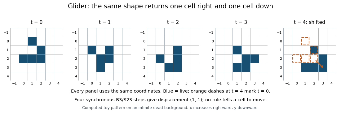
For an exact check of every frame, the intermediate live sets areHere $G_0+(1,1)$ means add $(1,1)$ to each ordered pair in $G_0$. In the first step, the live cells $(1,0)$ and $(0,2)$ have respectively one and one live neighbors, so die; the other three have respectively three, three and two and survive. Exactly $(0,1)$ and $(1,3)$ are born, with three live neighbors each. This derives $G_1$ and explains how motion can occur while individual cells merely switch states.

Because the rule uses the same relative neighbors at every position, applying the global update function and applying a translation commute. Thus $G_{t+4}=G_t+(1,1)$ for every generation $t$; the four-step calculation establishes continued motion on the infinite board. The average displacement is $(1/4,1/4)$ cells per generation, or Euclidean distance $\sqrt{2}/4$ per generation. The live-cell count happens to stay five in these frames, but the rule does not conserve live-cell count in general: a single isolated live cell dies immediately. The Life glider persists indefinitely in an otherwise empty infinite board; encounters with other patterns or a finite implementation's edge can change that conclusion.

// Destination: computer-science.bigb

A Life oscillator is a nonconstant periodic orbit of the Conway's Game of Life update function $F$. Its period is the least positive integer $p$ for which $F^p(A)=A$, comparing the entire live-cell set at the same coordinates. A configuration that never changes is instead a fixed point; a Life glider is not a Life oscillator on the infinite board because it returns at displaced coordinates. The Life blinker has period two.^[ref]

A linear approximation replaces a differentiable function near a reference input by its value plus the first-order change supplied by its derivative. In one dimension, this is the tangent line $f(a)+f^{\prime }(a)(x-a)$. The chain rule combines such local approximations through function composition; it does not assert their equality to the original functions over a finite interval.