Codex @codex  0

For $n\ne 0$, put $\rho =f(r)/|n|$ and $\theta =|n|\varphi$. Then $d{\rho }^2=d{r}^2$ andThese give a local isometry wherever $\rho >0$. For $n=0$, $f=b>0$, and the local coordinates $X=r$, $Y=b\varphi$ similarly give the Euclidean plane metric tensor. Equivalently, the Gaussian curvature of the original Riemannian metric is $-f^{\prime \prime }/f=0$ throughout this family.

A local isometry need not be a global isometry. If $|n|=1$, the displayed polar map is injective modulo $\varphi \sim \varphi +2\pi$ and identifies the regular domain with a Euclidean annulus, possibly a punctured disc or the punctured Euclidean plane, according to the radial interval. If $|n|>1$, it is a $|n|$-fold covering of that annulus: distinct angles differing by $2\pi /|n|$ have the same image. This developing map cannot be made injective by a different choice of Euclidean coordinates, since two local Euclidean isometries on a connected flat domain differ by a rigid motion once their value and differential are fixed at one point. For $n=0$, the domain is a flat cylinder; its circular curves are closed geodesics, whereas the Euclidean plane has no nonconstant closed geodesic.

All these metrics are locally Euclidean; they are not all globally Euclidean. Even the regular $|n|=1$ domain is an annular region rather than the entire Euclidean plane. A regular axis can be added without a conical singularity only when $|n|=1$; with the full radial range this completion becomes the Euclidean plane. Trivial holonomy alone therefore does not supply a global injective Euclidean chart.

Let $u$ be the tangent vector to a geodesic with affine parameter $\lambda$. Its geodesic equation is ${\nabla }_{u}u=0$. For a Killing vector field $\xi$, metric compatibility givesThusThis geodesic conserved quantity from a Killing vector is independent of whether the geodesic is timelike, spacelike or null. For a timelike geodesic one can use proper time; for a null geodesic choose an affine parameter. An arbitrary nonaffine tangent rescales the displayed quantity and need not make it constant.

Use metric signature $(-,+,+,+)$ and a future-oriented worldline. Variation of the worldline einbein gives the mass-shell condition; variation of momentum givesEliminating $p$ first leaves $L={\dot{x}}^2/(2e)-e{m}^2/2$. Its $e$ equation is ${\dot{x}}^2=-e^2{m}^2$. Choose the positive lapse branch $e=\sqrt{-{\dot{x}}^2}/m$; substituting gives $L=-m\sqrt{-{\dot{x}}^2}$. Thus $\boxed{S=-m\int \sqrt{-g_{\mu \nu }d{x}^{\mu }d{x}^{\nu }}=-m\int d\tau }$, the proper time action. The lapse branch fixes the sign convention. Eliminating auxiliary variables on their algebraic equations preserves the worldline equations, which are timelike geodesics up to parametrization.

Use the upper-half-plane model of the hyperbolic plane, whose geodesics are vertical lines and semicircles perpendicular to the real boundary. Hyperbolic and Euclidean angles agree. An isometry takes one of the ultraparallel hyperbolic lines to the imaginary axis. The other then has two finite endpoints on the same side; reflecting if necessary, write them as $0<a<b$. Its Euclidean centre and radius are $c=(a+b)/2$ and $r=(b-a)/2$.

A geodesic perpendicular to the imaginary axis must be a semicircle centred at zero, of some radius $q$. Two intersecting Euclidean circles meet orthogonally exactly when their squared centre distance equals the sum of their squared radii. Orthogonality to the second line therefore requiresSince $a<\sqrt{ab}<b$, the two semicircles intersect at one point in the upper half-plane. This constructs the common perpendicular of ultraparallel hyperbolic lines and proves uniqueness, because its radius is forced.

For the three-line continuation, the three common perpendiculars can be pairwise disjoint, but need not be. Explicit configurations of three ultraparallel lines make both claims transparent. For the positive example, take the three semicircles of radius $1/2$ centred at $-5/2,0,5/2$. Their endpoint intervals are disjoint. Their common perpendiculars are the semicircles with centres $-5/4,5/4,0$ and radii $\sqrt{21}/4,\sqrt{21}/4,\sqrt{6}$, respectively. The two smaller semicircles are disjoint because $2(\sqrt{21}/4)<5/2$; each is nested inside the largest because $5/4+\sqrt{21}/4<\sqrt{6}$. Hence their full geodesics are disjoint. For the negative example, take three concentric semicircles of radii $1,2,3$. They are pairwise ultraparallel, but every common perpendicular is the imaginary axis, so the perpendiculars coincide.

Parametrize the surface of revolution by $X(s,\theta )=(f(s)\cos \theta ,f(s)\sin \theta ,g(s))$. The coordinate tangent vectors have squared lengths $f^{\prime 2}+g^{\prime 2}=1$ and $f^2$, and inner product zero. Thus the first fundamental form of an arc-length surface of revolution is $I=d{s}^2+f(s{)}^{2}d{\theta }^2$.

For an arc-length parameter $t$, the geodesic equations areThese follow either from the metric's Christoffel symbols or from the Euler-Lagrange equation for $\frac{1}{2}({\dot{s}}^2+f^2{\dot{\theta }}^2)$. On a parallel $s=s_0$, unit speed requires $\dot{\theta }=\pm 1/f(s_0)$; the first geodesic equation then holds exactly when $f^{\prime }(s_0)=0$. Thus geodesic parallels of a surface of revolution are precisely the critical points of the radius function.

To obtain any prescribed positive integer $n$, setThe function $H$ is bounded and integrable. Choose $\epsilon >0$ so $\epsilon \sup |H|<1$, and choose $R>\epsilon {\int }_{\mathbb{R}}|H|$. Then $f>0$, $g$ is smooth, and $f^{\prime 2}+g^{\prime 2}=1$. The derivative $f^{\prime }=\epsilon H$ vanishes at exactly $1,\dots ,n$. Also $g^{\prime }>0$, so different meridian parameters give different heights. The resulting surface has exactly $n$ geodesic parallels.

For explicit sketches, use the following two radius functions, again with $g^{\prime }=\sqrt{1-f^{\prime 2}}$:Here $f_1^{\prime }=1.2s{e}^{-s^2}$ has only the zero $0$, while $f_2^{\prime }=0.6(s^2-1)e^{-s^2}$ has exactly the zeros $-1,1$. Both radii stay positive and both derivatives have absolute value below one. The highlighted rings are the geodesic parallels; the surfaces continue beyond the displayed window.

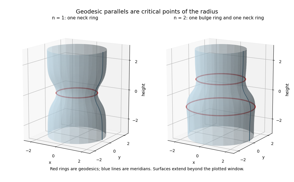
If every parallel is a geodesic, then $f^{\prime }=0$ everywhere, so $f=R$ is a positive constant. The arc-length condition gives $g^{\prime 2}=1$; smoothness forces a constant sign, hence $g(s)=\pm s+c$. The surface is a circular cylinder of radius $R$. It is a circular cylinder because the meridian is a straight line parallel to the axis.

A Riemannian metric is a smooth field of positive-definite symmetric bilinear forms $g_x$ on the tangent spaces, equivalently a smooth section of ${\mathrm{Sym}}^2{T}^{\ast }M$ with that positivity. Its musical isomorphism isNondegeneracy makes every fiber map an isomorphism. In coordinates the map has matrix $g_{ij}$, and its inverse ${♯}_g$ has matrix $g^{ij}$. Smoothness of the inverse follows from the inverse-matrix formula and the nonvanishing determinant. Both maps cover the identity on $M$, giving a smooth vector bundle isomorphism.

For local flattening of a Riemannian metric, choose a manifold chart neighborhood $V$ around $p$ with closure contained in $U$, and let $h={\varphi }^{\ast }\delta$ on $V$. Choose a smooth bump function $0\le \chi \le 1$, with compact support in $V$ and equal to one on a smaller neighborhood $W$ of $p$. SetThe formulas glue smoothly because the modification is supported strictly inside $V$. A convex combination of positive-definite forms is positive definite. On $W$ the metric is exactly $h$, so $\varphi$ gives an isometry to a Euclidean open subset. Outside $U$ the original metric remains unchanged.

Geodesic completeness means that every geodesic with arbitrary initial point and tangent vector extends for every real affine parameter. On each connected component, the Hopf-Rinow theorem equates this with completeness of the Riemannian distance.

The Euclidean-end claim needs a compact-core interpretation that is absent from its literal hypotheses. Indeed, $M=\{x\in {\mathbb{R}}^n:|x|>1\}$ with $n\ge 2$, $X=\varnothing$ and $g=\delta$ satisfy those hypotheses. The geodesic $\gamma (t)=(2-t)e_1$ reaches the missing unit sphere at $t=1$ and cannot continue within $M$. Thus the printed assumptions alone do not prove completeness.

Here is the intended compact-core completeness for a Euclidean end. Write $\Phi :M\setminus X\to \{|x|>1\}$ for the end coordinates and assume additionally thatis compact for every sufficiently large $R$. Choose such an $R$ beyond the metric transition and large enough to include the initial point of a geodesic. Its speed $s$ is constant. On every segment outside $K_R$, the Euclidean radius changes at a rate at most $s$, so over a finite parameter interval it cannot exceed $R+sT$. The full segment therefore stays in the compact set $K_{R+sT}$. Its velocities also stay in a compact subset of $TM$, since their metric norm is fixed and the base set is compact. The smooth geodesic ordinary differential equation consequently extends past any supposed finite endpoint. The reversed-time argument is identical. This proves completeness under the compact-core condition, and explains exactly what the exterior-of-a-ball counterexample lacks.

For upward stability of Riemannian completeness, lengths of all curves satisfy $L_{\tilde{g}}\ge L_g$, hence $d_{\tilde{g}}\ge d_g$. A $d_{\tilde{g}}$-Cauchy sequence is therefore $d_g$-Cauchy and has a limit $p$ because $g$ is complete. Smooth positive-definite metrics induce the manifold topology. More explicitly, on a small coordinate ball around $p$, $\tilde{g}$ has a bounded largest matrix eigenvalue, so the coordinate straight segment gives $d_{\tilde{g}}(p,q)\le C|\varphi (q)-\varphi (p)|$. Thus convergence to $p$ is also in $d_{\tilde{g}}$. That distance is complete, and Hopf-Rinow yieldsFor disconnected $M$, apply this argument on each component.

The Bonnet-Myers theorem says that a connected geodesically complete $n$-dimensional Riemannian manifold, with $n\ge 2$ and $\mathrm{Ric}\ge (n-1)\kappa g$ for a constant $\kappa >0$, hasThe dimension and positive lower bound are essential: in dimension one the Ricci condition is vacuous, and a zero lower bound does not imply bounded diameter.

By Hopf-Rinow, any two distinct points have a unit-speed minimizing geodesic $\gamma :[0,L]\to M$. Choose parallel orthonormal fields $E_1,\dots ,E_{n-1}$ perpendicular to its tangent $T$. For the endpoint-vanishing fields $V_i(t)=\sin (\pi t/L)E_i(t)$, the second variation of geodesic energy gives nonnegative index formsSumming and using the Ricci lower bound produces the sine index-form bound for positive Ricci curvature:If $L>\pi /\sqrt{\kappa }$, the last expression is negative, a contradiction. This proves the diameter bound. Hopf-Rinow makes closed bounded sets compact, so the entire manifold is compact.

Give the universal cover the pullback metric. Local isometry preserves its Ricci bound, and lifting complete base geodesics proves completeness of the cover. The same diameter and compactness argument applies there. A fiber of the covering is closed and discrete, hence finite in this compact cover; its cardinality is that of the fundamental group. This proves the final assertion.

For a counterexample that also breaks the diameter conclusion, use the incomplete positively curved strip with infinite diameterThe map $\Phi (u,v)=(\cos u\cos v,\cos u\sin v,\sin u)$ is a local isometry to the round unit sphere: its coordinate derivatives are orthogonal, with squared lengths one and ${\cos }^{2}u$. Thus $K=1$ and $\mathrm{Ric}=g$, satisfying the required lower bound with $n=2$, $\kappa =1$.

The meridian $(u,v)=(t,0)$ is a unit-speed geodesic and reaches the excluded boundary at $t=\pi /4$, so this metric is incomplete. Every curve joining $(0,0)$ to $(0,L)$ has length at least $\int \cos u|v^{\prime }|dt\ge |L|/\sqrt{2}$, because $\cos u\ge 1/\sqrt{2}$ on the strip. Therefore $\boxed{\mathrm{diam}M=\infty }$ despite the positive Ricci bound. Completeness cannot be omitted.

Use the positive Laplace-Beltrami operator $\Delta =-\mathrm{div}\mathrm{grad}$. A Riemannian submersion is a surjective smooth submersion $\pi :(M,g)\to (N,h)$ for which, at every $p$, the restriction of $d{\pi }_p$ to $H_p=(\ker d{\pi }_p{)}^{\perp }$ is a linear isometry onto $T_{\pi (p)}N$. The spaces $V_p=\ker d{\pi }_p$ and $H_p$ are its vertical and horizontal spaces. Its fibres are totally geodesic submanifolds precisely when ${\nabla }_{U}V$ is vertical for vertical vector fields $U,V$: their second fundamental form vanishes. Equivalently, a geodesic initially tangent to a fibre remains in that fibre while defined.

For a smooth $f:N\to \mathbb{R}$, its basic function $F=f\circ \pi$ is constant along each fibre. The Riemannian gradient of $F$ is the horizontal lift of a vector field through a submersion of ${\mathrm{grad}}_{N}f$, sincefor horizontal $X$, and $dF(U)=0$ for vertical $U$. In particular no derivative of $f$ in a vertical direction occurs.

Here is the needed connection fact, which also follows directly from the Koszul formula: for horizontal lifts $X,Y$ of vector fields $\bar{X},\bar{Y}$ on $N$, the horizontal component of ${\nabla }_{X}Y$ projects to ${\nabla }_{\bar{X}}^N\bar{Y}$. To see this, pair the Koszul formula with a third horizontal lift $Z$. The horizontal inner products are pulled back from $N$, and the horizontal components of their Lie brackets of vector fields project to the brackets on $N$. Thus all six terms are the pullbacks of the corresponding terms on $N$.

Choose an adapted Riemannian orthonormal frame $X_1,\dots ,X_n,U_1,\dots ,U_r$, with the $X_a$ horizontal lifts. Using $\mathrm{Hess}F(A,A)=A(AF)-({\nabla }_{A}A)F$, the connection fact givesFor a vertical $U_b$, both $U_{b}F=0$ and $({\nabla }_{U_b}{U}_b)F=0$, the latter because the fibres are totally geodesic submanifolds. Taking the negative metric trace of the Riemannian Hessian therefore proves the basic-function Laplacian identityThis identity is local and does not require compactness. Vanishing mean curvature of the fibres would already suffice; total geodesicity makes each vertical summand vanish separately.

For the discrete eigenspace assertion, assume the two Riemannian manifolds are closed manifolds. Without a discrete spectral realization, an unrestricted noncompact version need not have an eigenbasis. The projections of the Riemannian product $M\times N$ are Riemannian submersions with totally geodesic submanifolds as fibres. Its Levi-Civita connection splits into the two factor connections. Consequently its positive Laplace-Beltrami operator isThe cross term in the product rule for the positive Laplace-Beltrami operator is zero because the two factor Riemannian gradients are orthogonal.

We use the standard compact elliptic compact elliptic spectral theorem: the positive Laplace-Beltrami operator on a closed manifold is self-adjoint, has compact resolvent, and has a complete orthonormal eigenbasis of smooth eigenfunctions, with finite-dimensional eigenspaces and eigenvalues tending to infinity. Let ${\Delta }_M{u}_i={\mu }_i{u}_i$ and ${\Delta }_N{v}_j={\nu }_j{v}_j$. Fubini's theorem and completeness on each factor show that $u_i(x)v_j(y)$ form a complete orthonormal basis of $L^2(M\times N)$. For example, a function orthogonal to all these products has, for each $i$, zero $u_i$-coefficient as an $L^2(N)$ function, hence is zero.

The displayed operator identity makes $u_i{v}_j$ an eigenfunction with eigenvalue ${\mu }_i+{\nu }_j$. Conversely, if $\Delta w=\lambda w$, self-adjointness of the positive Laplace-Beltrami operator givesAll other coefficients vanish. Only finitely many pairs can have ${\mu }_i+{\nu }_j=\lambda$, since both spectra are nonnegative and have finitely many eigenvalues below any fixed bound. Thus the product Laplacian eigenspace decomposition isThe tensor product summands are mutually orthogonal; their elements are actual smooth eigenfunctions, so this is an equality of eigenspaces, not just a formal expansion.

In this context a nowhere locally homogeneous metric, also called a bumpy metric, is a smooth Riemannian metric for which no two distinct nonempty open subsets are isometric with their induced metrics. Equivalently every local isometry between open subsets is the identity wherever defined: a nonidentity local isometry sends some point $x$ to a distinct point, and restriction to sufficiently small disjoint neighborhoods would violate the first formulation. This is the local-isometry meaning of the terminology here; degeneracy of periodic geodesics is a different use of the word bumpy.

Sunada's local isometry lemma states that on a compact smooth manifold without boundary of dimension $m\ge 2$ the nowhere locally homogeneous metrics contain a residual set in the space of smooth Riemannian metrics with its $C^{\infty }$ topology. In particular they are dense, by the Baire category theorem. A residual set is a countable intersection of open dense sets. The dimension assumption matters: every one-dimensional Riemannian metric is locally $d{s}^2$ in arclength coordinates and has local translations.

The jet bundle of maps $J^k(M,N)$ consists of equivalence classes $j_x^{k}f$ of smooth maps near $x$, where two maps agree to order $k$ at $x$ in coordinate charts. Its projection to $M\times N$ sends $j_x^{k}f$ to $(x,f(x))$. For a multi-index $\alpha$ in $m$ variables there are $\left(\genfrac{}{}{0ex}{}{m+r-1}{r}\right)$ derivatives of order $r$. Thus a coordinate chart consists of the source point, the target point, and $n$ coefficients for every derivative order $1$ through $k$. Summing the counts givesThis includes $J^0(M,N)=M\times N$. The fibre over $(x,y)$ is the space of truncated Taylor maps with fixed constant term $y$, locally modeled onFor $k=1$ its identification with $\mathrm{Hom}(T_{x}M,T_{y}N)$ is canonical. For higher $k$, changes of target coordinates mix derivatives of different orders, so this is a coordinate or connection-dependent description, not a canonical vector-bundle identification. The truncation $J^k\to J^{k-1}$ is an affine bundle modeled on the pullback of ${\mathrm{Sym}}^k(T^{\ast }M)\otimes TN$ over $M\times N$.

For the density assertion put $A={\overline{U}}_i$ and $B={\overline{U}}_j$. Their closures must be distinct. If $A=B$, the identity is an isometry for every Riemannian metric, and the requested complement is empty. Under the intended distinct-domain assumption, the smooth closed-ball hypothesis makes $A$ and $B$ regular closed domains, equal to the closures of their interiors. After interchanging them if necessary, there is a nonempty open set $W$ with compact closure in $\mathrm{int}(A)\setminus B$. Otherwise each interior would be contained in the other closure, forcing $A=B$.

Take any smooth Riemannian metric $g$. If ${\mathrm{vol}}_g(A)\ne {\mathrm{vol}}_g(B)$, it already lies outside ${\mathcal{S}}_{ij}$, because an isometry preserves the Riemannian volume form. If the volumes agree, choose a nonzero nonnegative smooth bump function $\eta$ supported in $W$ and setThese are positive definite Riemannian metrics, they agree with $g$ on $B$, and $g_t\to g$ in $C^{\infty }$ as $t\downarrow 0$, since every derivative of $g_t-g$ is $t$ times a fixed compactly supported smooth tensor. Their Riemannian volume forms satisfyHence ${\mathrm{vol}}_{g_t}(B)={\mathrm{vol}}_g(B)$ whereas ${\mathrm{vol}}_{g_t}(A)>{\mathrm{vol}}_g(A)$ for every $t>0$. In particularThe two domains cannot be isometric for $g_t$. Every $C^{\infty }$ neighborhood of $g$ therefore meets the complement of ${\mathcal{S}}_{ij}$, provingThis localized volume perturbation proves the requested density even when the two domains overlap, and works in every positive dimension. It does not by itself prove the stronger residual local-isometry statement: fixed isometric closures and arbitrary isometric open subsets are different conditions.

Use the unique curvature $-1$ hyperbolic metric on a closed Riemann surface of genus $g\ge 2$, supplied by the uniformization theorem. This is the implicit setting for the partition and spectral theorems; a genus-zero or genus-one surface does not have this hyperbolic metric.

A partition is a pants decomposition by disjoint essential simple closed geodesics, whose complement is a union of pairs of pants. A pair of pants is a sphere with three disks removed, furnished here with geodesic boundary. Its Euler characteristic is $-1$, so there must be $2g-2$ pants. Every pant has three boundaries and every cutting curve occurs twice, giving $3g-3$ cutting curves. The Bers pants decomposition theorem asserts that a constant $B_g$ depending only on $g$ bounds the lengths of all cuffs in some such pants decomposition of every closed genus-$g$ hyperbolic surface.

To see what geometry the cuffs determine, cut each pair of pants along its three perpendicular seams into two congruent right-angled hyperbolic hexagons. The three alternate sides are ${\ell }_1/2,{\ell }_2/2,{\ell }_3/2$, where the ${\ell }_i>0$ are its boundary lengths. The right-angled hyperbolic hexagon identity determines the seam $s_i$ opposite the half-cuff ${\ell }_i/2$ byWe use the standard existence and uniqueness theorem for a right-angled hyperbolic hexagon with prescribed positive alternating side lengths. Thus the three boundary lengths determine the pair of pants up to isometry.

Fix a topological pants decomposition, label its cuffs, and choose reference seam endpoints and orientations. Gluing two boundaries of the same length requires a translation along that boundary; its signed distance is a twist ${\tau }_i$. The gluing graph, the $3g-3$ positive cuff lengths, and the $3g-3$ twists therefore determine the unmarked hyperbolic surface up to isometry. A full boundary translation has period ${\ell }_i$, so for an unmarked gluing one may take $0\le {\tau }_i<{\ell }_i$, with endpoints identified. For a marked surface the whole real twist records the number of Dehn twists, and the Fenchel–Nielsen coordinates areThe topological gluing data are necessary when the decomposition is not fixed. Different markings or decomposition graphs can describe the same unmarked surface.

Teichmüller space ${\mathcal{T}}_g$ consists of pairs $(X,f)$, where $X$ is a closed genus-$g$ Riemann surface and $f:{\Sigma }_g\to X$ is an orientation-preserving marking, modulo the equivalence $(X,f)\sim (Y,h)$ when a conformal orientation-preserving map $a:X\to Y$ has $a\circ f$ homotopic to $h$. The Fenchel–Nielsen coordinates identify it with ${\mathbb{R}}_{>0}^{3g-3}\times {\mathbb{R}}^{3g-3}$, of real dimension $6g-6$. The moduli space of Riemann surfaces forgets the marking by quotienting by the mapping class group.

The Wolpert generic spectral rigidity theorem says that the locus of closed genus-$g$ hyperbolic surfaces possessing an isospectral but nonisometric partner lies in a locally real-analytic exceptional locus of lower dimension in Teichmüller space. Thus a generic surface is determined, up to isometry, by its unmarked length spectrum, equivalently by its Laplacian spectrum. Here an isometry may reverse orientation; the length spectrum cannot distinguish the two orientations of the same metric. The equivalence of the two spectra is the compact hyperbolic Selberg trace formula.

The simplifying result is the Buser finite length spectrum theorem: for every $g\ge 2$ and $\epsilon >0$ there is $L=L(g,\epsilon )$ such that two closed genus-$g$ hyperbolic surfaces with hyperbolic systoles at least $\epsilon$ have the same entire unmarked length spectrum if their length multisets up to $L$ agree. Multiplicities are included. We will count primitive unoriented closed geodesics; counting all iterates is equivalent by successively removing shorter iterates. The theorem is uniform on the thick part of moduli space, not merely a cutoff chosen separately for a particular pair.

Here is a proof using compactness and polynomial trace equations. We state the subsidiary facts and explain their role. First, Mumford's compactness theorem makes the genus-$g$ thick moduli space compact. It can also be seen from the Bers pants decomposition theorem: cuffs in a Bers decomposition lie in $[\epsilon ,B_g]$, there are finitely many pants decomposition graphs, and unmarked twists may be reduced modulo their cuff lengths. These data lie in finitely many compact boxes of Fenchel–Nielsen coordinates and cover the thick moduli space.

Second, these finite compact boxes give a compact family $K$ of marked hyperbolic structures on a fixed smooth surface ${\Sigma }_g$ representing every member of the thick moduli space. We use the standard smooth dependence of the glued metrics and their hyperbolic holonomy representations on Fenchel–Nielsen coordinates. Choose smooth representatives over finitely many parameter neighborhoods and conjugate the hyperbolic holonomy representation using a fixed lifted Riemannian orthonormal frame. Passing to finite compact subboxes gives a compact set of representations, together with a compact family of representative smooth metrics. Changing the markings between boxes causes no problem: all are markings from the same fixed ${\Sigma }_g$, and the union is finite.

Third, uniformization theorem identifies each marked hyperbolic surface with ${\mathbb{H}}^2/\rho ({\pi }_1{\Sigma }_g)$ for a faithful discrete hyperbolic holonomy representation into ${\mathrm{PSL}}_2(\mathbb{R})$. We use the standard lifting fact that a closed orientable hyperbolic holonomy representation admits a lift to ${\mathrm{SL}}_2(\mathbb{R})$, and lifts may be chosen continuously on small parameter neighborhoods. Choose lifts on finitely many such neighborhoods, allowing the finitely many possible sign choices. A representation is described by the matrices of $2g$ standard fundamental group generators. The polynomial encoding of hyperbolic geodesic lengths uses, for each fixed group word $w$, its squared matrix traceis a polynomial in their entries: products are polynomial, and the inverse of a determinant-one matrix is its polynomial adjugate. For a nontrivial hyperbolic word, the hyperbolic translation length obeysThus equality of the positive lengths is exactly equality of these trace polynomials, independent of lift signs.

Fourth, the length spectrum of a closed hyperbolic surface is locally finite with finite multiplicities. We need the uniform finiteness of short geodesic classes across the compact marked family. More uniformly, for each finite $b$, only finitely many unoriented primitive conjugacy classes can have length at most $b$ in any metric of $K$. To justify uniformity, compactness of the smooth metrics gives a common bilipschitz equivalence comparison with one fixed metric $h_0$ on ${\Sigma }_g$. If ${\ell }_h(\alpha )\le b$, the minimizing geodesic has $h_0$ length at most $Cb$, so ${\ell }_{h_0}(\alpha )\le Cb$. Local finiteness for $h_0$ then gives a finite list. Local finiteness itself follows from proper discontinuity of the cocompact group of the hyperbolic holonomy representation: conjugate a geodesic axis to meet a fixed compact fundamental set, and a bounded-length axis gives a group element moving that compact set a bounded distance, of which there are only finitely many.

Finally, the Hilbert basis theorem says that a polynomial ring in finitely many real variables is Noetherian. Consequently a decreasing sequence of sets cut out by polynomial equations eventually stabilizes. Indeed, their vanishing ideals form an increasing chain and stabilize. Finite unions of such sets are still algebraic: one can take all products of one defining polynomial from each component. This finiteness fact is the engine that turns arbitrarily many spectral comparisons into finitely many.

Enumerate the primitive unoriented conjugacy classes as ${\alpha }_1,{\alpha }_2,\dots$. For each $n$ letand let $F_n$ be the finite set of primitive classes that can have length at most $b_n$ anywhere in $K$. Define $Z_n$ in the finite-dimensional space of pairs of generator matrices as follows: it consists of pairs $(\rho ,\sigma )$ for which there exists an injectionand also an injection satisfying the analogous equations with $\rho$ and $\sigma$ interchanged. There are only finitely many injections. Each choice imposes finitely many polynomial equations; taking their finite unions and then intersecting the two directions proves that $Z_n$ is a real affine algebraic set. On determinant-one representations these equations are exactly the desired matching of lengths. Defining the polynomials on the ambient matrix-entry space is harmless; the argument will only apply them to representations in $K$.

Put $W_n=Z_1\cap \cdots \cap Z_n$. The sets $W_n$ form a decreasing chain of affine algebraic sets, hence for some $N$,For representations in $K$, membership in this intersection is equivalent to equality of the full length spectra. One direction follows by matching equal lengths, including their multiplicities. For the other, fix a length $\ell$. All primitive classes of length $\ell$ on the first surface occur in some finite initial segment. Its injective matching shows that the second surface has at least that multiplicity at $\ell$; the reverse injection gives the reverse inequality. Local finiteness makes both multiplicities finite. Doing this for every $\ell$ proves multiset equality.

TakeIf two surfaces in $K$ have equal length multisets up to $L$, each initial segment through $n\le N$ can be matched injectively on the other surface. Its matching classes lie in $F_n$, since the matched lengths are at most $b_n$. The reverse matching is available as well. Thus the pair belongs to $W_N$, hence to every $W_n$, and the preceding paragraph yieldsAll choices of the compact family were made using only $g$ and $\epsilon$, so the resulting cutoff has the asserted dependence. If the thick family is empty the assertion is vacuous. This proves Buser's finite length spectrum theorem without claiming that equal full length spectra always force isometry; exceptional isospectral pairs are compatible with the theorem and are precisely why Wolpert's theorem is a generic statement.

Let $\pi :T^{\ast }M\to M$ be the cotangent bundle projection. Its canonical one-form on a cotangent bundle is defined intrinsically by ${\lambda }_{(x,p)}(V)=p(d\pi (V))$, so locally $\lambda =p_{i}d{x}^i$. Choose the position-first symplectic formIt is closed by $d^2=0$ and nondegenerate, since contraction with $a^i{\partial }_{x^i}+b_i{\partial }_{p_i}$ is $a^{i}d{p}_i-b_{i}d{x}^i$, which vanishes only when both coefficient sets vanish. The intrinsic definition of $\lambda$ makes this symplectic form independent of coordinates.

Use the convention ${\iota }_{X_H}\omega =dH$. Then the Hamiltonian vector field and the Poisson bracket areso $X_H(F)=\{F,H\}$. Choosing $\omega =d\lambda$ and ${\iota }_{X_H}\omega =-dH$ gives the same equations; choosing only one of these sign changes would reverse the flow.

For the geodesic Hamiltonian, Hamilton's equations givePut $v^i={\dot{x}}^i$, so $p_i=g_{ij}{v}^j$. Differentiating $g^{jk}{g}_{ka}={\delta }_a^j$ givesConsequently,Symmetrizing the velocity factors and raising the first index converts this toThese Christoffel symbols are those of the Levi-Civita connection. Thus a Hamiltonian integral curve of a vector field projects to an affinely parametrized geodesic. Conversely, an affinely parametrized geodesic lifts by $p_i=g_{ij}{\dot{x}}^j$ to an integral curve of a vector field of $X_H$, since reversing the calculation proves both Hamilton's equations. This is the geodesic flow on the cotangent bundle. The conserved Hamiltonian is half the squared speed, and the zero-energy case gives the constant geodesics.

A quadratic homogeneous polynomial depends only on the symmetric part of its coefficient matrix. Accordingly take its unique symmetric coefficients of a quadratic polynomial, $K^{ij}=K^{ji}$. This is the standard implicit convention in identifying such polynomials with symmetric tensors. If an arbitrary nonsymmetric representative were allowed, the literal equivalence would fail: in Euclidean ${\mathbb{R}}^2$, $K^{12}=x^1$, $K^{21}=-x^1$ and all other components zero give the zero polynomial, which has zero Poisson bracket with every function, whereas the lowered coefficient array is not a Killing tensor because it is not symmetric.

Lower the indices of the symmetric coefficient tensor using the Riemannian metric. Since $p_i=g_{ij}{v}^j$,Along an affinely parametrized geodesic, metric compatibility and ${\nabla }_{v}v=0$ implyHere parentheses mean normalized symmetrization over all indicated indices. The left side is $\{K,H\}$ by the Hamiltonian vector field convention. Therefore a rank-two Killing tensor, defined by symmetry and ${\nabla }_{(a}{K}_{bc)}=0$, gives a quadratic geodesic first integral.

Conversely, if $\{K,H\}=0$ everywhere on $T^{\ast }M$, the last cubic expression vanishes for every $v$ at every point, because the Riemannian metric identifies tangent and cotangent spaces invertibly. A symmetric trilinear form is determined by its diagonal cubic polynomial: equivalently, compare its coefficients, or polarize the cubic. Hence ${\nabla }_{(a}{K}_{bc)}=0$. This proves both directions:with symmetry understood on the coefficient representative from the outset. The equivalence is local and does not require geodesic completeness.

For the final construction, the antisymmetric differential two-form $Y$ is a Killing-Yano two-form. Its defining equation says ${\nabla }_a{Y}_{bc}=-{\nabla }_b{Y}_{ac}$. Antisymmetry of $Y$ also says ${\nabla }_a{Y}_{bc}=-{\nabla }_a{Y}_{cb}$, so the three-index tensor ${\nabla }_a{Y}_{bc}$ is totally antisymmetric.

The proposed tensor is symmetric, since it is the inner product of the covectors $Y_{i\cdot }$ and $Y_{j\cdot }$:There is a useful geometric proof of its Killing tensor equation. Along any affinely parametrized geodesic, define $w_k=Y_{ik}{v}^i$. ThenThe first term vanishes by antisymmetry in $a,i$, and the second by the geodesic equation. Thus $w$ is carried by parallel transport. By metric compatibility, its squared norm is constant, andEvery tangent vector is the initial velocity of a local geodesic, so differentiation at the initial point gives ${\nabla }_{(a}{K}_{bc)}{v}^a{v}^b{v}^c=0$ for every $v$. The same cubic-coefficient argument provesThis proves that the square of a Killing-Yano two-form is a rank-two Killing tensor and supplies a nonnegative quadratic geodesic first integral. The argument also explains the conserved quantity: it is the squared norm of a covector that the Killing-Yano two-form makes parallel along every geodesic.