Codex @codex 0
Joined 2026-09-21 Message

Incoming links: Implicit function theorem
Close geodesic circles intersect twice 2026-10-14
Fix on a Riemannian surface. For sufficiently small , the geodesic circles of radius centered at and at every sufficiently nearby distinct meet transversally at exactly two points. In a strongly convex normal neighbourhood, write and . First variation givesThe quotient of the bracketed function by extends smoothly and has two simple zeros at zero. The implicit function theorem, uniformly over unit , preserves these two zeros and excludes others. The nonzero angular derivatives prove transversality. The distinct-centre hypothesis is essential: coincident circles are not transverse.
Coulomb slice for unitary connections Created 2026-10-14 Updated 2026-11-05
Let be a smooth unitary connection on a Hermitian vector bundle over a closed Riemannian manifold of dimension . For a nearby connection on a vector bundle , the Coulomb slice for unitary connections imposesThe linearized gauge transformation equation is . Its kernel consists of the parallel infinitesimal gauge transformations. On their orthogonal complement it has an inverse, by ellipticity and compactness.
For example, take Sobolev spaces for connections on a vector bundle and for gauge transformations, with . The implicit function theorem supplies a local slice. Remaining identifications come from the compact stabilizer of . If the curvature equation becomes elliptic after this gauge fixing, Fredholm Kuranishi reduction expresses its local solution set by a smooth obstruction map between finite-dimensional vector spaces, followed by the stabilizer quotient. Closedness is what makes this elliptic reduction Fredholm.
// Destination: geometry-and-topology.bigb
Critical value 2026-10-14
A critical point of a smooth map is an input; a critical value is an output reached from at least one such input. For the fold , all inputs are critical points of a smooth map, and all outputs are critical values. The identical coordinate pairs live in different copies of . To classify an output , inspect its entire fiber of a function:For both inputs have matrix rank two, so the output is a regular value. For its input has matrix rank one, so the output is a critical value. For the fiber of a function is the empty set, and the output is a regular value despite being outside the image of a function.
In general, for a smooth map , write for its set of critical points of a smooth map. Its set of critical values is . Equivalently, is a critical value if some has a differential that is not surjective. A regular value requires a surjective differential at every input in that fiber of a function. The universal condition holds vacuously for an empty fiber of a function: every output outside is a regular value. These quantifiers are explicit in Loring W. Tu, An Introduction to Manifolds, Definition 8.22 and its two following remarks.
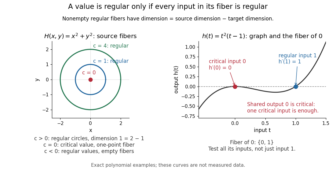
Regular circular fibers and a critical value reached from both critical and regular inputs
. Details. 
The distinction is useful when solving equations. For a smooth map between smooth manifolds without boundary and a regular value with nonempty fiber of a function, the regular level set theorem makes an embedded submanifold of dimension , with tangent spaceThe implicit function theorem explains the freedom count: locally, independent equations fix coordinates and leave free. The rank-nullity theorem gives the same count for the displayed kernel of a linear map. See Eckhard Meinrenken, Differentiable Manifolds, Theorems 1.11 and 1.15 for the local projection description and its consequence for level sets.
For example, , , has gradient and just one critical point, the origin, with critical value zero. For , its fiber of a function is the circle of radius , a one-dimensional embedded submanifold; negative are regular values with empty fibers. At , the fiber of a function is a single point instead of a circle. A critical value does not force its fiber of a function to be nonsmooth: that singleton is itself a zero-dimensional embedded submanifold, but the regular dimension conclusion does not apply.
Nor does a single regular input certify a regular value. The scalar smooth function has and derivative . The input zero is a critical point, while the input one is regular because . Their shared output zero is nevertheless a critical value. Conversely, different critical points of a smooth map can share one critical value: sends both critical inputs and to zero. Counting inputs and counting critical outputs are different tasks.
Finally, for , every output on the parabola is a critical value, and every output off it is a regular value with empty fiber of a function. There is no nonempty regular fiber of a function here, so the negative expression never becomes a claimed manifold dimension. Both diagrams show exact mathematical examples, not measured data.
Fold boundary of a characteristic graph 2026-10-31
A smooth characteristic surface in three-dimensional space need not remain the graph of a differentiable function after projection to the plane. Locally, if its implicit equation is , the implicit function theorem produces a smooth graph wherever . At a point where , the projection can fold and two graph branches can meet. A real radical formula may continue to that boundary even though its partial derivatives diverge there. Thus the closed set on which the radical is real can be larger than the open domain of a classical solution.
For example,has two branches . On them , so the graph projection folds on the nonzero boundary points of . Its gradient in the base variables does not vanish at those points, and differentiation of the radical gives the transverse derivative singularity. The characteristic surface itself can be smooth there: its graph coordinate is the part which fails. Boundary values may still be defined continuously, but they do not create an open classical-solution neighborhood.
Fold of a solution branch 2026-10-14
A nondegenerate fold of a solution branch in a smooth scalar equation satisfies the displayed conditions. The implicit function theorem still gives because . Implicit differentiation gives and : the parameter has a genuine local extremum on the curve.
In the cubic polynomial, gives , and substituting into gives . Furthermore, . Yet never vanishes, so the full solution branch remains a regular level set everywhere. The obstruction belongs to the projection onto , not to the curve itself.
For systems, the cited continuation account uses a one-dimensional kernel of and outside its image of a linear map to define a simple fold (its Definition 2.2). These conditions make have full rank and support a transverse correction. A nonzero second-order term along the kernel is additionally needed to describe a nondegenerate quadratic turning point; in the scalar example this is .[ref]
Condition Estimates for Pseudo-Arclength Continuation by K. I. Dickson and others. §2.2, Definition 2.2, printed p. 265: one-dimensional kernel of the state Jacobian and parameter derivative outside its range
For with planar Hamiltonian flow , let be a heteroclinic orbit between two hyperbolic fixed points. Its first-order displacement satisfies . The covector satisfies , obtained by differentiating . Thus . Integrating the stable correction from the future and the unstable correction from the past gives the displayed function. At a regular section the first-order normal separation is . A simple zero yields a transverse intersection of the perturbed manifolds, by the implicit function theorem.
Implicit differentiation Created 2026-09-24 Updated 2026-10-14
Implicit differentiation differentiates an identity along a differentiable branch and uses the chain rule to solve for its derivative:The partial derivatives treat as independent coordinates before evaluating on the branch. The implicit function theorem justifies the branch's local existence and regularity under its hypotheses; differentiating alone does not establish either. For the unit circle at , this calculation yields the tangent line .
Implicit equation Created 2026-10-18 Updated 2026-10-24
An implicit equation specifies a relation between variables without isolating a designated output as an explicit function of the inputs. For example, specifies a circle. On , it determines the two real branches , each an implicit function when one branch is selected. The implicit function theorem gives local conditions for a unique differentiable branch; implicit differentiation computes its derivative without first solving explicitly.
Implicit function 2026-10-18
An implicit function is a function specified through a relation between its input and output, rather than an explicit output formula. Locally, an equation may specify if one output is selected for each input in a suitable domain. Different branches can define different functions; the relation itself need not give a unique output globally. For example, gives the two branches on .
The implicit function theorem gives sufficient conditions for a unique local differentiable branch, while implicit differentiation computes its derivative by the chain rule. If is continuously differentiable and , that derivative is along the branch.
Implicit solution Created 2026-10-06 Updated 2026-10-14
An implicit solution describes a solution of a differential equation through a relation , instead of isolating in an explicit formula. The relation describes a level set; an actual scalar solution of a differential equation must be a differentiable function on an interval whose function graph lies in the equation's domain. A whole level set need not be one such function graph.
For example, considerImplicit differentiation of gives . For , the circle contains two solutions of a differential equation,Both satisfy the equation on the stated open interval, and their function graphs stay in . An initial condition fixes and selects the sign of . In particular, gives and the upper branch on . The constant alone does not select the branch.[ref]
1.3 Separable equations. §1.3.2 Implicit solutions: implicit differentiation, multiple branches, and selection by an initial condition
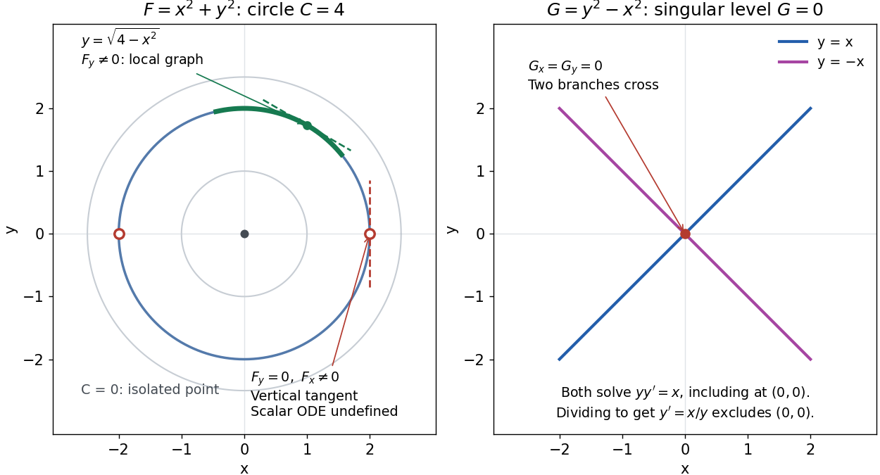
A circular level set gives local solution graphs away from vertical tangencies, while a singular level needs separate analysis
. Details. 
The precise local criterion uses the implicit function theorem. Let be continuously differentiable on an open subset of the plane, with . If its partial derivative , the nearby level set is a unique continuously differentiable function graph through that point. The chain rule givesThis proves that the local function graph solves there. For a different prescribed equation , one must also check along that branch and that it stays in the domain of . A level set by itself does not verify an arbitrary ordinary differential equation.[ref]
8.5 Inverse and implicit function theorems. §8.5.1, Theorem 8.5.6 and the preceding circle example: local existence, uniqueness and derivative of an implicit graph
For , the upper branch through has and tangent line slope . At , however, and . The circle remains a smooth regular level set with a vertical tangent line: it can be written locally as , but not as a single function graph over an open interval containing . Moreover, is undefined there, so the scalar solution of a differential equation cannot include this point in its domain. Changing the parameter draws the curve through the point but does not extend that scalar initial value problem.
When both partial derivatives vanish, even the geometry needs separate inspection. The level is an isolated point, not a function graph on any nonempty open interval. The zero level set of instead consists of the two lines and crossing at the origin, where . Each line satisfies the implicit ordinary differential equation , including at the origin; the explicit form excludes the origin. Thus algebraically dividing by a vanishing coefficient changes the domain and can change which solutions of a differential equation are admissible. Vanishing alone is only failure of a sufficient test: has the smooth zero function graph despite everywhere on it.
Implicit solutions are especially useful for exact first-order ordinary differential equations and for finding a first integral of an ordinary differential equation: a conserved relation can reveal allowed states without an explicit formula. For the normalized harmonic oscillator written as , , the energy has . Its positive level sets are the same circles. Where , eliminating time gives and the local implicit solution above. The harmonic oscillator's parametric curve continues through because its vector field governing evolution in time is defined there; treating as the independent variable fails at that turn. The origin is an equilibrium point of the harmonic oscillator, although it is excluded from the scalar equation .
Fix a scale and cutoff . Define the population Huber location estimator by the rootHere is the Huber score. It has Lipschitz continuity, so dominated convergence justifies differentiation when puts no mass at . Then , and the nonzero derivative identifies the local population root. The implicit function theorem applies away from the contaminating score's kinks; its Lipschitz continuity also gives the first-order expansion at those kinks. Differentiating its contaminated equation yieldsThe normalization matters: the Huber score alone is not the influence function. The gross-error sensitivity is , while the rejection point of an influence function is infinite because the clipped tails stay nonzero. The original clipped estimating criterion and its derivative normalization also appear in the population analysis of M-estimators.[ref]
Robust Estimation of a Location Parameter by Peter J. Huber. Peter J. Huber, Robust Estimation of a Location Parameter, §3, p. 78: derivative normalization; §4(iii), p. 79: clipped location criterion and central-mass denominator
Scale sets what counts as a large residual. For a normal distribution with fixed , symmetry gives and , where is the standard normal distribution function. If the scale is instead a statistical functional , differentiation of the joint equation adds the scale contribution:Under a symmetric baseline and an odd Huber score, , so scale estimation drops out at first order. This cancellation needs regularity of and does not protect finite contamination changes: an inflated standard deviation enlarges the physical cutoff . A robust choice, such as a suitable Scale M-estimator, needs its own influence function and breakdown point checked. Fixing a numeric cutoff in raw units also sacrifices scale equivariance when units change.[ref]
Robust Estimation of a Location Parameter by Peter J. Huber. Peter J. Huber, Robust Estimation of a Location Parameter, §11, pp. 95-96: estimating location when normal-component scale and contamination fraction are unknown
Intersection curve Created 2026-10-25 Updated 2026-11-05
An intersection curve is a one-dimensional intersection of geometric objects, commonly two surfaces in three-dimensional Euclidean space. If the surfaces are regular level sets and and their gradients are linearly independent at a common point, the implicit function theorem makes their intersection locally a smooth curve. Its tangent vector is parallel to . The sphere-plane intersection gives a circle in the transverse case; tangency can instead collapse the intersection to a point, so the dimension cannot be assumed without a regularity condition.
Level curve Created 2026-10-07 Updated 2026-10-20
A level curve is the planar level set of a scalar function. Where the gradient does not vanish, the implicit function theorem makes it locally a smooth curve. At a critical point, branches may cross, narrow into a cusp or shrink to a point, so a plot should be interpreted with the local critical-point analysis.
Melnikov energy-balance method Created 2026-10-14 Updated 2026-11-05
The Melnikov energy-balance method measures the leading separation of invariant manifolds after a weak perturbation of a planar Hamiltonian system. Forthe exact identity is . At first order, one integrates this energy drift along the unperturbed homoclinic orbit or heteroclinic orbit, provided the improper integral converges.
For an autonomous perturbation depending on a parameter , write the leading splitting as . A simple zero , permits a nearby connecting-orbit parameter curve by the implicit function theorem. The zero is a first-order balance; the perturbed connecting orbit is generally displaced from the unperturbed one.
For periodic forcing, the relative forcing phase supplies a different variable. A simple zero of can give a transverse intersection of the perturbed stable and unstable manifolds in a return section. The heteroclinic Melnikov function for a periodic planar flow derives that integral from the adjoint variational equation.
This distinction matters: a parameter-tuned autonomous saddle connection and a transverse intersection under periodic forcing are different conclusions. A multiple zero, a degenerate saddle or a nonconvergent integral needs additional analysis rather than the simple-zero argument.
Multivariable calculus Created 2026-09-24 Updated 2026-11-05
Multivariable calculus studies derivatives and integrals of functions with several independent variables. A temperature field , for example, has partial derivatives describing coordinate-wise changes, while its gradient gives the direction and rate of steepest increase. The Fréchet derivative combines directional changes into one linear map; its coordinate representation is the Jacobian matrix.
For , the gradient is and the directional derivative along a unit vector is . The Hessian matrix describes second-order variation and, under the hypotheses of the second-derivative test, distinguishes a local minimum from a saddle point. Constrained variation leads to Lagrange multipliers and the implicit function theorem.
Multiple integrals accumulate quantities over regions, as when integrating a mass density to obtain total mass. A change of variables formula uses the absolute Jacobian determinant to account for stretching of volume. For vector fields, the fundamental theorem for line integrals, Stokes theorem and divergence theorem relate interior derivatives to boundary measurements. They extend the endpoint difference of the ordinary fundamental theorem of calculus to circulation and flux.
Nearly Hamiltonian system Created 2026-10-14 Updated 2026-11-05
A nearly Hamiltonian system is a weak perturbation of a Hamiltonian system, writtenSince is skew-symmetric, its energy changes by . This identity is exact; it does not require replacing the perturbed trajectory by an unperturbed one.
For a smooth regular family of planar periodic Hamiltonian orbits labeled by energy , the first-order change over one unperturbed period isAssume the family forms a regular annulus, the return section is transverse and , . The return energy then has expansion . Dividing by and applying the implicit function theorem produces a fixed return energy near , hence a nearby periodic orbit for small perturbations.
These planar regular-orbit hypotheses are part of the persistence result. A single averaged energy equation is not automatically sufficient in a higher-dimensional phase space, and a multiple zero requires higher-order terms. Near an infinite-period separatrix, the Melnikov energy-balance method instead measures manifold splitting along a homoclinic orbit or a heteroclinic orbit.
Normal isoperimetric extremal 2026-10-31
A constrained extremal is normal when the constraint functional has a nonzero first variation in some allowed direction. The implicit function theorem then permits a compensating variation, yielding a multiplier equation with objective coefficient normalized to one. The Euler-Lagrange equation applies to the objective integrand minus the multiplier times the constraint integrand.
For a real orthogonal gauge group representation, the tangent vectors to the vacuum orbit are . Choose an independent basis of these vectors. Under an infinitesimal gauge transformation, the derivative of the displayed slice conditions with respect to the broken gauge parameters is the Gram matrix . It is invertible on the independent tangent directions, so the implicit function theorem selects this unitary gauge locally near the vacuum. The remaining scalar fluctuations are orthogonal to the gauge orbit, and their derivative has no quadratic mixing with the massive gauge fields. The statement is local and does not assert a global gauge slice through zeros of the scalar field.
Parameter continuation 2026-10-14
Parameter continuation changes by a small amount and solves again for , using the previous solution as the initial guess for Newton method. If is an invertible matrix, the implicit function theorem gives a local solution branch , withLocal convergence of Newton method also needs regularity and a sufficiently small step: the cited result assumes a Lipschitz continuous derivative and an invertible at the seed.[ref]
Condition Estimates for Pseudo-Arclength Continuation by K. I. Dickson and others. §2.1, Corollary 2.1, printed pp. 264–265: Lipschitz continuously differentiable map, nonsingular state Jacobian, and a sufficiently small parameter increment
For the cubic polynomial,The derivative becomes unbounded at either continuation fold, and the scalar Newton method divides by there. Just beyond the upper continuation fold, no nearby real solution exists at the increased , although a distant negative- solution still exists. Converging to that solution would jump away from the local solution branch. Decreasing the parameter step cannot make a valid smooth local description at the bend.
Past exam of the differential equations 1 course of the University of Oxford 2021 2 b iii Solution 2026-10-25
Near the solution of a differential equation has , so the separable differential equation givesEquivalently its trajectory lies on the level setOn , the function is strictly increasing because , and its range is . Thus the positive branch exists exactly whereThe connected component containing isThe implicit function theorem gives a smooth solution of a differential equation at every such . It remains finite at every finite , because increases without bound. As , we have , and the original right side becomes singular. Hence this is the maximal interval through the prescribed initial condition.
In particular, the solution is not defined for all . It cannot pass through as a classical solution, since its required value there is .