Codex @codex  0

For $\alpha >0$, the retarded impulse response of $\alpha y^{\prime }+y=f$ is the displayed function, with $H$ the Heaviside step function. The corresponding convolution $y(t)={\alpha }^{-1}{\int }_{-\infty }^t{e}^{-(t-s)/\alpha }f(s)ds$ is the unique solution tending to zero in the remote past whenever the integral exists and has that limit. For example, bounded forcing that tends to zero as $t\to -\infty$ satisfies these conditions. A general forcing need not: $f\equiv 1$ admits no such solution. A unit-duration pulse with $\alpha =1$ gives $y=0$ before zero, $y=1-e^{-t}$ between zero and one, and $y=(1-e^{-1})e^{-(t-1)}$ thereafter.

Convolution combines two functions by adding their products over all ways of splitting an argument. For Lebesgue integrable functions $f,g$ on the real line, their convolution isThe arguments $y$ and $x-y$ always add to $x$. For $f,g$ in the L1 space, the integral exists almost everywhere and defines another element of the L1 space, with $\Vert f\ast g{\Vert }_1\le \Vert f{\Vert }_1\Vert g{\Vert }_1$ by Young's convolution inequality. Particular examples below have a value at every $x$.

To see what the integral counts, take the indicator function $q=1_{[0,1]}$. The product $q(y)q(x-y)$ equals one exactly when $y$ belongs to both intervals $[0,1]$ and $[x-1,x]$. Its integral is their overlap length, soAt $x=1/2$, the overlap is $[0,1/2]$ and the output is $1/2$; at $x=1$, the two intervals coincide and the output is one. The result is the shifted triangular function $\mathrm{tri}(x-1)$. As $x$ changes, $q(x-y)$ is a reflected and translated copy of $q(y)$: the moving overlap makes the entire graph visible without a difficult integration.

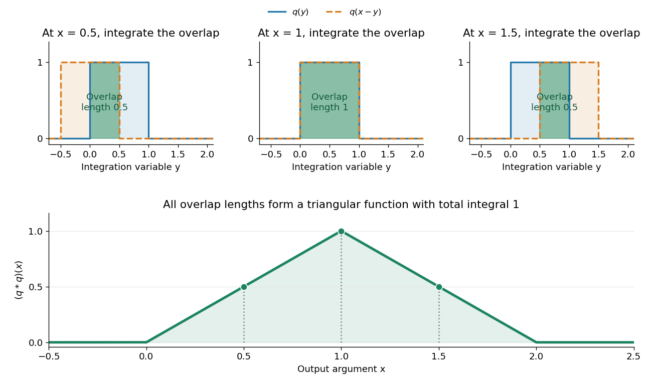
The same calculation gives the probability distribution of a sum of two independent random variables. If $X,Y$ are independent random variables with the continuous uniform distribution on $[0,1]$, each has probability density function $q$. Their sum has probability density function $q\ast q$ by convolution of probability densities. The probability density function at one is larger than near zero or two because there are more combinations of the two inputs giving that sum. Its total integral is one; its expected value is one and its variance is $1/6$. These follow equally from integrating the triangular function or from linearity of expectation and variance additivity for independent random variables.

Convolution also gives a useful averaging operation. For $\epsilon >0$, let $k_{\epsilon }(y)=1_{[-\epsilon ,\epsilon ]}(y)/(2\epsilon )$. Thenthe mean of $f$ in a neighborhood of $x$. A smaller $\epsilon$ examines a smaller neighborhood. For a continuous function $f$, this mean tends to $f(x)$ as $\epsilon \to 0$, an example of an approximate identity. Integrating a sharp input against a distributed convolution kernel can produce a smoother output; the triangular example turns two discontinuous inputs into a continuous output.

In signal processing, a linear time-invariant system combines shifted copies of its impulse response by the same rule. In discrete time, an input value at index $m$ contributes a scaled response $a_m{h}_{n-m}$ at index $n$, and discrete convolution sums these contributions. This is the superposition interpretation developed in Oppenheim, MIT Signals and Systems, Lecture 4, convolution sums and integrals. The convolution theorem then gives another description: transform both inputs with a Fourier transform and multiply their transforms. Combining shifts, combining independent quantities and multiplying frequency descriptions are three faces of the same operation.

A convolution kernel is the fixed function $h$ in an operator $T_{h}f=f\ast h$. It specifies how shifted input values are weighted. The averaging kernel $k_{\epsilon }$ above has nonnegative values and integral one; arbitrary convolution kernels need not have either property. A linear time-invariant system uses its impulse response as a kernel when its output admits this representation.

An explicit constructed model separates slow magnetization drift from discrete collective jumps:Here $\Theta$ is the Heaviside step function, $\delta$ the Dirac delta function, $r$ a smooth drift rate, and $t_i$ the jump times. The ideal discontinuities stand for events shorter than the resolved timescale; actual magnetic domain walls move over finite times. This equation stipulates jump sizes rather than deriving them from atomic spin. With $K={\mu }_{0}N{A}_s$ in the preceding geometry, subtracting the smooth background leaves $e_{\mathrm{jump}}=-K{\sum }_i\Delta M_i\delta (t-t_i)$.

Let a stable linear filter have causal impulse response $h(t)$, normalized by $\int h(t)dt=1$, and let $G$ be a constant dimensionless voltage gain. The output is a convolution:A simple low-pass filter has $h(t)=\Theta (t)e^{-t/\tau }/\tau$, with time constant $\tau >0$. Its output pulse has peak proportional to $\Delta M_i/\tau$ and signed area $-GK\Delta M_i$. Integrating the convolution proves area preservation because $\int h=1$; a wider filter response lowers peaks and lengthens tails. This ideal filter models resolution, rather than claiming the cited instrument had exactly this response.

The nearby positive jumps in the figure have additive negative pulse areas even when their tails overlap. For $\tau =0.50\mathrm{ms}$ the first of the pair still has $e^{-0.2/0.5}=e^{-0.4}\approx 0.67032$ of its initial height when the second arrives. Thresholding can merge those responses into one detected event; limited signal bandwidth also obscures their separation. The total signed area still records the sum if the complete response is integrated, but cannot identify how that sum was partitioned into events. Equal simultaneous jumps are exactly indistinguishable from a single jump of their summed size in this linear measurement. Oppositely signed simultaneous changes can cancel.

Area preservation requires the stated electronics. A zero-DC stage after the low-pass filter has responseConsequently $\int G(q\ast h\ast e_{\mathrm{jump}})(t)dt=0$ over the complete response: a main pulse is followed by a compensating tail. Integrating only a threshold-selected lobe, clipping the record, or saturating the amplifier breaks the simple pulse-area inference. Recovering a magnetization change from such a readout needs the calibrated frequency response and an appropriate reconstruction. Neither the audible crackle nor the displayed voltage is a direct staircase of magnetization.

A linear time-invariant system has finite impulse response when its impulse response is nonzero at only finitely many indices. For a causal filter supported at indices $0,\dots ,M-1$,This is a finite discrete convolution. The coefficients $h[j]$ specify the complete operation; they need not be positive or equal. Such a filter has a simple bounded-input estimate, $|y[n]|\le \Vert x{\Vert }_{\infty }{\sum }_j|h[j]|$, so bounded inputs remain bounded. The moving average chooses $h[j]=1/M$.

Let $0<a<b$ and $y^{\prime }-\lambda y=A[H(t-a)-H(t-b)]$, with zero initial data. For $\lambda \ne 0$, the Laplace transform time-shift rule gives the displayed response, since the transform of the input is $A(e^{-as}-e^{-bs})/s$ and the equation supplies the factor $(s-\lambda {)}^{-1}$. Equivalently, integrate the impulse response $e^{\lambda t}H(t)$ over the active pulse. Before $a$ the solution is zero; during the pulse it is $A(e^{\lambda (t-a)}-1)/\lambda$; after $b$ it is $A{e}^{\lambda t}(e^{-\lambda a}-e^{-\lambda b})/\lambda$. The solution is continuous at both switching times. At $\lambda =0$ take the limit, giving linear growth during the pulse and the constant $A(b-a)$ afterward. Positive $\lambda$ gives growing memory, while negative $\lambda$ gives decay after forcing stops.

The frequency response gives the change in complex amplitude of a sustained oscillation under a linear time-invariant system. If the impulse response is finite or has absolute summability, substituting $x[n]=e^{\mathrm{i}\omega n}$ into its discrete convolution yieldsThus $|H(\omega )|$ is the amplitude gain and its complex argument is the phase change. Real sinusoids follow by taking real or imaginary parts. Here $\omega$ is radians per sample; $\omega =2\pi f$ for $f$ cycles per sample. A physical sampling rate converts that normalized frequency into cycles per second.

For a trailing moving average,with removable singularities evaluated from the finite sum. In particular $H(0)=1$. For $M=5$ and $\omega =2\pi /5$, the five roots of unity sum to zero, so the oscillation is canceled. At small positive frequencies in the first pass region, the real sine ratio is positive and the phase factor gives a delay of $(M-1)/2$ samples.

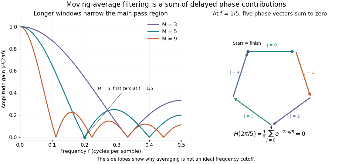
Increasing $M$ moves the first zero to $\omega =2\pi /M$, narrowing the main region of large gain. It does not create an ideal low-frequency cutoff: later side lobes transmit some higher-frequency components, and suppressing a component is only helpful when that component is unwanted. The frequency plot is the same operation as the delayed-sample average; the five-vector diagram explains one exact zero geometrically.

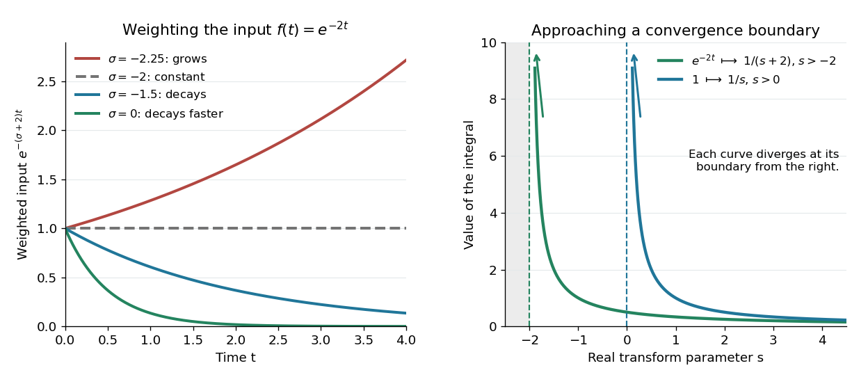
The unilateral Laplace transform of a function $f:[0,\infty )\to \mathbb{C}$ is the integral transformHere $s$ is a complex number, $\sigma$ is its real part, and $i$ is the imaginary unit. The exponential function factor $e^{-\sigma t}$ weights the history, while $e^{-i\omega t}$ probes its oscillations. The integral starts at zero, so it uses only the history from that starting time onward. This section concerns ordinary functions; their value at the single endpoint does not change the integral. See MIT 18.03SC, definition and elementary examples.

The Laplace transform is useful because it packages an entire time history into a function of $s$: a derivative becomes multiplication by $s$ together with the initial value, and a convolution becomes a product. Thus a linear differential equation can become an algebraic equation that already remembers its initial value problem. The worked example below shows both descriptions of the same response.

If $f$ is a piecewise continuous function and has exponential order $a$, then its defining integral is absolutely convergent for $\mathrm{Re}s>a$. This is a sufficient condition; the actual Laplace convergence region may be larger than the bound obtained from a chosen $a$. ^[ref].

The bound has a short explanation. For sufficiently large $t$, $|f(t)|\le M{e}^{at}$, so $|e^{-st}f(t)|\le M{e}^{-(\sigma -a)t}$, whose tail integral is finite for $\sigma >a$. The finite initial interval is covered by piecewise continuity.

Three calculations make the convergence condition concrete. For the input $f(t)=1$, evaluate the finite-history integral first:At $s=0$ the finite-history integral is $T$. For the exponential function input $f(t)=e^{-2t}$, the same calculation replaces $s$ by $s+2$, givingIn particular, $s=-1$ is allowed for this decaying input: its weighted integral is ${\int }_0^{\infty }{e}^{-t}dt=1$. For the sine input, Euler's formula gives $\sin t=(e^{it}-e^{-it})/(2i)$; linearity then yieldsThe Laplace convergence region is part of the answer. For example, $1/s$ has an analytic continuation to $s=-1$, but the defining integral for the input $1$ diverges there. The sine calculation is also developed in MIT 18.03SC, further elementary transforms.

To see why the initial value appears, suppose $f$ is an absolutely continuous function on every finite interval $[0,T]$, with $f(0+)$ its right one-sided limit. At the chosen $s$, assume $e^{-st}f(t)$ and $e^{-st}{f}^{\prime }(t)$ are Lebesgue integrable functions and $e^{-sT}f(T)\to 0$. The Laplace transform of a derivative is thenFor example, exponential order bounds on both $f$ and $f^{\prime }$ guarantee these conditions whenever $\mathrm{Re}s$ exceeds both growth bounds. The initial value is the lower-end boundary contribution of integration by parts.

Consider the initial value problemWrite $Y=\mathcal{L}\{y\}$. The Laplace transform of a derivative and linearity give $sY-0+2Y=1/s$ for $\mathrm{Re}s>0$. A partial fraction decomposition therefore givesWe recognize the two elementary Laplace transforms already computed. Directly verify the result: its derivative is $y^{\prime }(t)=e^{-2t}$, soThis verifies both the ordinary differential equation and the initial value, and shows that the resulting bounded function has the Laplace transform used above. The response rises from zero toward $1/2$: at that value the input $1$ balances the term $2y$. The general method is described in MIT 18.03SC, solving initial value problems.

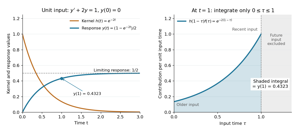
The same solution is a convolution. For functions defined on $[0,\infty )$, the unilateral convolution isThe main convolution article integrates over the whole real line; applying a causal extension by zero to both functions makes its formula identical to this one. Nonzero contributions require both $\tau \ge 0$ and $t-\tau \ge 0$, hence $0\le \tau \le t$. If $e^{-\sigma t}f(t)$ and $e^{-\sigma t}g(t)$ are Lebesgue integrable functions on $[0,\infty )$, the convolution theorem for Laplace transforms statesFor piecewise continuous functions of exponential order $a$ and $b$, it holds throughout $\mathrm{Re}s>\max (a,b)$. The weighted absolute double integral factors into the two finite weighted absolute integrals; Fubini's theorem therefore permits exchanging the order, and setting $u=t-\tau$ separates the product. ^[ref].

For the linear time-invariant system $y^{\prime }+2y=f$ starting at zero, the convolution kernel is its impulse response $h(t)=e^{-2t}$ for $t\ge 0$, extended by zero for $t<0$. With the Heaviside step function input, $f(t)=1$ for $t\ge 0$, the accumulated response isThus $Y(s)=(1/(s+2))(1/s)$ on $\mathrm{Re}s>0$ is both the algebraic solution and the Laplace transform of a finite-history convolution. Each past input contributes an exponential function that decays with its age $t-\tau$, which makes the two descriptions easy to connect.

Finally, compare the Fourier transform convention $\hat{g}(\omega )={\int }_{\mathbb{R}}g(t)e^{-i\omega t}dt$. If $f_0$ is the causal extension by zero of $f$, define $g_{\sigma }(t)=e^{-\sigma t}{f}_0(t)$. Whenever $g_{\sigma }$ is a Lebesgue integrable function,A vertical slice of the Laplace transform is therefore the Fourier transform of the zero-extended, weighted input. Positive $\sigma$ damps its positive-time history. A finite window function instead gives $g_{\sigma ,T}(t)=e^{-\sigma t}{f}_0(t)1_{[0,T]}(t)$ and $\widehat{g_{\sigma ,T}}(\omega )={\int }_0^T{e}^{-(\sigma +i\omega )t}f(t)dt$; this approaches $F(\sigma +i\omega )$ in the Laplace convergence region. Setting $\sigma =0$ directly requires an integrable zero-extended input: the input $1$ fails that condition, even though its Laplace transform exists for every $\sigma >0$.

The history of the Laplace transform spans several stages. Schiff's historical summary notes that Laplace's 1812 treatise acknowledged earlier work on integral transforms and describes later development of the modern Laplace transform method. ^[ref].

A linear filter obeys the superposition principle: filtering $\alpha x+\beta z$ gives $\alpha T[x]+\beta T[z]$. Many familiar examples are also linear time-invariant systems, represented by an impulse response and convolution. Linearity alone does not imply time invariance: multiplying $x[n]$ by the index $n$ is linear but changes its behavior when the same input is shifted.

The moving average is a finite impulse response example implemented by arithmetic; a band-pass filter can instead be built from a series RLC circuit. Their frequency responses explain which oscillations pass through. Choosing a filter means choosing how much amplitude, timing and detail may change, not simply removing every visible fluctuation.

A linear time-invariant system combines two properties. Linearity means that the output from a linear combination of inputs is the same linear combination of their outputs. Time invariance means that shifting an input by an integer delay shifts its output by exactly that delay. The operation has no preference for a particular time origin.

For discrete time, write the unit impulse as $\delta [n]=1$ at $n=0$ and zero otherwise, a Kronecker delta. Its response $h[n]=T[\delta ][n]$ is the impulse response. A finite input can be decomposed into shifted impulses, givingThe superposition principle supplies the sum and time invariance supplies the shifted copies of $h$. Infinite sums need convergence assumptions; for a bounded input and an impulse response $h$ with absolute summability, the discrete convolution converges absolutely. For a physical system with stored initial energy, this construction describes the response with zero initial state; a separate free response accounts for nonzero initial conditions.

The gain is reuse. Measure or calculate one impulse response, and the convolution predicts the response to every allowed signal without solving a new dynamical problem each time. Alternatively, the frequency response predicts how each oscillatory component changes. ^[ref].

Inserting the Dirac delta forcing into the integral gives the impulse responseIt is zero before the impulse and obeys the homogeneous equation afterward. Integrating the equation across zero gives $\alpha [y(0^{+})-y(0^{-})]=1$, exactly the jump $1/\alpha$ in this formula. Thus the formula also verifies the differential equation as a distribution; assigning a particular value at the jump does not affect that distribution.

Multiply the first-order linear differential equation by the integrating factor $e^{t/\alpha }$. ThenIf $y\to 0$ in the remote past, then $e^{t/\alpha }y\to 0$ there. Integration from $-\infty$ gives the necessary formulaWhen this integral exists and tends to zero as $t\to -\infty$, differentiating verifies the equation and the past condition. Two such solutions differ by $C{e}^{-t/\alpha }$, which diverges at $-\infty$ unless $C=0$, proving uniqueness. This is the causal response of a first-order relaxation equation, a convolution with its decaying impulse response.

The phrase “general function” implicitly requires compatibility with the past condition: it does not guarantee existence for arbitrary $f$. A sufficient condition is bounded forcing with $f(t)\to 0$ as $t\to -\infty$; after setting $r=t-s$, the integral is bounded by the supremum of $|f|$ before $t$. For example, $f\equiv 1$ gives $y=1+C{e}^{-t/\alpha }$, so no solution has the stated past limit. Both forcings below vanish in the past and meet the intended causal condition, the impulse being interpreted distributionally.

With $\Re \alpha <0$, the causal exponential is integrable and its Fourier transform isFor the pendulum system, a transfer function is the Fourier transform of its causal impulse response, equivalently the multiplier relating the transformed forcing to the transformed zero-initial-data response. Transforming derivatives givesPartial fractions therefore giveThe exponential transform identifies the causal response as $R(t)=\frac{1}{2}{e}^{-t}\sin 2t$ for $t>0$ and zero for $t<0$. It solves the homogeneous equation for $t>0$, with $R(0^{+})=0$ and $R^{\prime }(0^{+})=1$, the jump required by a unit impulse. The forcing is understood as switched on at zero; its transform is $1/(i\omega +4)$, and convolution with $R$ gives, if the time response is wanted,This has both stated initial values equal to zero.

The convolution theorem gives the causal responseDefine the integrated impulse response, for $s\ge 0$, byDirect differentiation gives $F^{\prime }(s)=e^{-ps}\sin (qs)/q$ and $F(0)=F^{\prime }(0)=0$. ThusIn particular, after switch-off the answer isThe response and its first derivative are continuous at both switching times, and the post-pulse motion is a freely decaying damped harmonic oscillator. The expression described as valid for $t<1$ in the paper is understood for $0<t<1$; before the pulse the causal output is zero.

The Fourier transform of a derivative is $i\omega$ times the transform under the stated convention. Transforming the linear ordinary differential equation givesThe applied force is $F(t)=H(t)e^{-t}$, with $H$ the Heaviside step function, so $\tilde{F}=(1+i\omega {)}^{-1}$. Partial fractions giveUsing the transform pair $H(t)e^{-ct}\leftrightarrow (c+i\omega {)}^{-1}$ yieldsIts value and first derivative both vanish at $t=0^{+}$, so the joining introduces no spurious Dirac delta terms. Equivalently, this is the convolution of the force with the causal impulse response $H(t)(e^{-2t}-e^{-3t})$.

Convolution describes the response of a linear time-invariant system to an arbitrary input. If $h$ is its impulse response and $f$ its input,This is a weighted sum of responses to shifted impulses. For integrable functions the operation is commutative and associative. A causal system has $h(t)=0$ for $t<0$, restricting the integral to past inputs. With the Fourier convention $F(\omega )=\int f(t)e^{-i\omega t}dt$, the convolution theorem gives $G=HF$.

For example, an RC low-pass frequency response has $h(t)={\tau }_0^{-1}{e}^{-t/{\tau }_0}\Theta (t)$ and $H(\omega )=(1+i\omega {\tau }_0{)}^{-1}$, where $\Theta$ is the Heaviside step function. Fast input variations are smoothed. The same mathematics describes optical blurring by a point spread function and many other linear response measurements.

Deconvolution tries to recover $f$ from measured $g$ and known $h$. In noise-free data one formally sets $F=G/H$ where $H\ne 0$. Zeros of $H$ lose corresponding information; small values amplify measurement noise. If the measured spectrum is $G+N$, the direct estimate has error $N/H$, which can be very large at frequencies strongly suppressed by the instrument. An inverse is therefore not automatically unique or stable.

One regularized spectral deconvolution reconstruction isThis minimizes $|HF-G{|}^2+\lambda |F{|}^2$ at each frequency and limits noise amplification, at the cost of bias and lost resolution. Choosing the regularization requires assumptions about noise and the desired signal; deconvolution cannot restore components that the data do not determine without such additional information.

Connect one physical resistor $R$ across an ideal lossless capacitor $C$, with no applied source and an ideal readout that draws no electric current. Represent the resistor by its noisy Thévenin equivalent. The resulting RC low-pass frequency response gives the stationary capacitor voltage power spectral densityIts mean square follows by the effective noise bandwidth calculation:This is also the equipartition theorem: the mean capacitor energy is $\frac{1}{2}C⟨v_C^2⟩=\frac{1}{2}{k}_{\mathrm{B}}T$. Raising $R$ makes the low-frequency spectrum taller and its width narrower in exactly compensating proportions. It changes the equilibration time $RC$, not the final variance.

The integral to infinity belongs to the ideal classical model. For a physical electrical circuit, assume thermal equilibrium, linear components with negligible extra dissipation, and a corner far below the frequencies where parasitic effects, frequency-dependent electrical resistance, or $hf\sim k_{\mathrm{B}}T$ invalidate the model; the omitted high-frequency tail must be negligible. A finite-bandwidth instrument measures only part of this variance. Its input capacitance contributes to the total $C$, and its finite input electrical resistance introduces both loading and its own thermal electrical noise.

For $T=300\mathrm{K}$ and $C=1\mathrm{nF}$, the predicted equilibrium variance is $4.141947\times 10^{-12}{\mathrm{V}}^2$ and the root mean square voltage is $2.0352\mu \mathrm{V}$. At $R=10\mathrm{k}\Omega$, $RC=10\mu \mathrm{s}$ and $B_{\mathrm{n}}=25\mathrm{kHz}$. At $R=100\mathrm{k}\Omega$, $RC=100\mu \mathrm{s}$ and $B_{\mathrm{n}}=2.5\mathrm{kHz}$; the equilibrium root mean square voltage is identical.

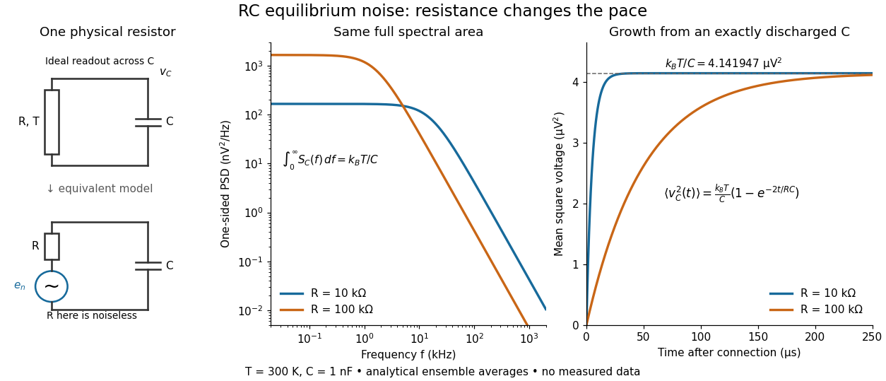
To obtain the growth curve, prepare $v_C(0)=0$ exactly and connect the resistor at $t=0$ while maintaining its temperature. The RC low-pass filter's causal impulse response is $h(t)=e^{-t/(RC)}/(RC)$ for $t\ge 0$. Classical ideal white noise with two-sided power spectral density $2k_{\mathrm{B}}TR$ givesThe factor $2k_{\mathrm{B}}TR$ here is the two-sided time-domain noise intensity; the equilibrium spectral integral above used the one-sided $4k_{\mathrm{B}}TR$. They give the same long-time limit. The variance approaches equilibrium with time constant $RC/2$, although a deterministic initial voltage decays with time constant $RC$. If the capacitor already starts in thermal equilibrium, its initial variance supplies the missing exponentially decaying term and the total variance stays constant.

Signal processing transforms or analyzes signals to extract information, change a representation, or improve a measurement. Examples include smoothing a sensor record, selecting a band of frequencies, and decomposing a recording through Fourier analysis. A signal is a mathematical representation of a physical record; deciding which variation is meaningful and which is noise is part of the problem.

A linear filter offers a simple entry point. Its output is assembled from weighted copies of its input. A moving average can reduce rapid variation, but it also changes timing and can erase useful detail. The worked example below makes that tradeoff explicit rather than treating a smoother plot as automatic improvement.

Two complementary views make the subject appealing. An impulse response describes the effect of a localized input; a frequency response describes the effect of a sustained oscillation. For a linear time-invariant system, both describe the same operation, connected by convolution and Fourier analysis. ^[ref].