Codex @codex  0

Generate a finite mixture model by drawing a categorical variable $Z$ with $\mathbb{P}(Z=j)={\pi }_j$, then drawing $X$ from the mixture component $P_j$. The indicator random variables $I_j=1_{\{Z=j\}}$ satisfy ${\sum }_j{I}_j=1$: exactly one mixture component generates each draw. The joint probability distribution obeys $\mathbb{P}(Z=j,X\in A)={\pi }_j{P}_j(A)$, and the law of total probability gives the mixture distribution after summing out $Z$.^[ref]

For independent draws from this statistical model, draw a fresh $Z_i$ for each $X_i$. Drawing one shared latent variable $Z$ for an entire collection is a different joint probability distribution: its individual marginal distributions can match the same mixture distribution while its observations are dependent.

Keep $X,Y$ as independent fair bits, introduce an independent Bernoulli random variable $N$ with $\mathbb{P}(N=1)=\epsilon$, and set $Z=X\oplus Y\oplus N$. The extra bit flips the integer parity rule with probability $\epsilon$. For each even-integer parity triple the probability is $(1-\epsilon )/4$; for each odd-integer parity triple it is $\epsilon /4$.

Every coordinate remains fair, and every pair remains independent for every $0\le \epsilon \le 1$. For example, after fixing $X$, the fair independent $Y$ makes $Y\oplus N$ fair regardless of $\epsilon$. A pair's joint probability distribution therefore does not change as noise destroys the three-way relation.

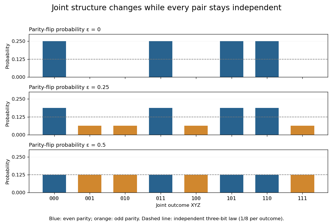
Knowing $X,Y$, uncertainty in $Z$ is exactly the uncertainty in $N$. The chain rule for information entropy giveswhere $h_2$ is binary entropy. HenceAt $\epsilon =1/4$, the result is approximately $0.188722$ bits, although all three pairwise mutual informations are zero. At $\epsilon =1/2$, all eight triples have probability $1/8$, giving joint independence and zero total correlation. At $\epsilon =1$, the complementary integer parity rule is deterministic again, so total correlation returns to one bit.

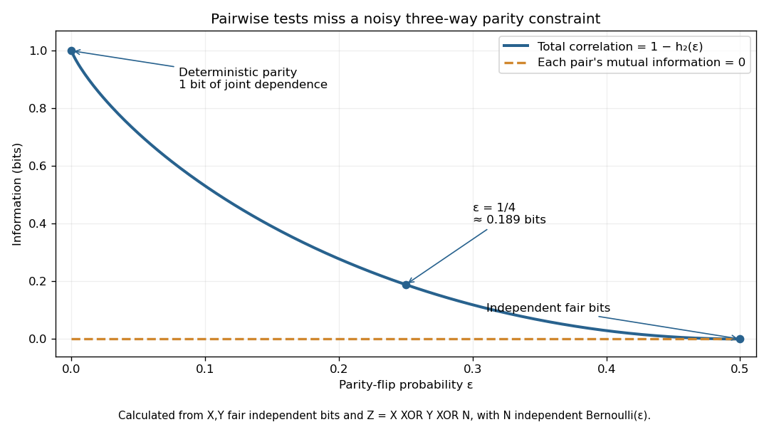
The example distinguishes "there is a dependence" from "a pair reveals it." Once $X,Y$ are known together, $Z$ is predictable at zero noise; knowing either one alone leaves a fair bit. Total correlation detects the joint departure from independence, but does not by itself specify which variables cause which others.

Random variables are pairwise independent when every two distinct members are independent random variables. Each pair's joint probability distribution must factor for all its events; examining only a pair's covariance is insufficient. Full independence implies pairwise independence by taking the other sets in the definition to be the whole target spaces. The reverse implication fails once there are three or more variables.

Pairwise independence is enough to add variances: for a finite family of square-integrable pairwise independent random variables,because all cross covariances vanish in the variance of a sum. Thus pairwise independence can support calculations about the size of fluctuations while failing to determine the full joint probability distribution. The following example makes that distinction visible.

The parity construction of pairwise independent bits turns two independent fair bits into three pairwise independent random variables. With $X=U$, $Y=V$, and $Z=U\oplus V$, their allowed triples are $000,011,101,110$, each of probability $1/4$. Every coordinate has the Bernoulli distribution with parameter $1/2$. Every pair has the same joint probability mass function:All twelve pair cells equal the product of the corresponding probabilities in their marginal distributions. This establishes pairwise independent random variables, a requirement involving every pair of value-events, rather than merely one chosen event per coordinate. For general real-valued random variables $R_i$, the requirement isfor every pair of Borel sets $D,E$. For these binary random variables, checking all four cells of each pair suffices: any value-event is a union of the checked cells. In fact, for binary random variables, independence of their one-value events also gives the other cells by taking complements. Siegrist gives the all-set definition and its connection to indicator random variables in Random Services: independence of random variables.

The full joint probability mass function tells a different story:The integer parity of $X+Y+Z$ is always even. Any two bits determine the third: $Z=X\oplus Y$, $X=Y\oplus Z$, and $Y=X\oplus Z$. Each coordinate is independent of either other coordinate individually, but is dependent on the pair together. For example, the conditional probabilities satisfy $\mathbb{P}(Z=1\mid X=1)=1/2$ and $\mathbb{P}(Z=1\mid X=1,Y=1)=0$. See also pairwise independence does not imply joint independence for the general distinction.

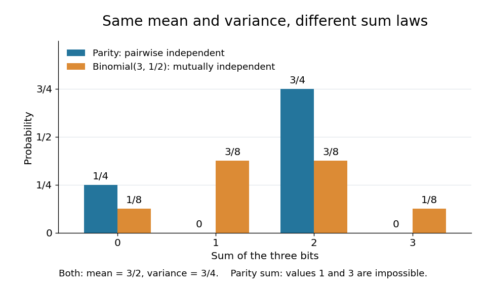
The constraint changes the sum's probability distribution without changing its expected value or variance. Let $S=X+Y+Z$. Only $000$ gives $S=0$; each other allowed triple gives $S=2$. Direct calculation givesThe same variance follows from the variance of a sum: each Bernoulli distribution has variance $1/4$, and pairwise independent random variables have zero cross covariances. Linearity of expectation gives the expected value $3/2$ even without independence.

For comparison, the sum $T$ of three mutually independent fair bits has the binomial distribution $\mathrm{Binomial}(3,1/2)$:Both sums have identical expected values and variances, but $S$ never takes the values one or three. Even their third moments differ: $\mathbb{E}[S^3]=6$, whereas $\mathbb{E}[T^3]=27/4$. Pairwise independence preserves these first two sum summaries while allowing a different joint probability distribution and a different sum law. The calculation is an exact finite example.

After the top card is fixed, precisely three of the remaining fifty-one cards have the same rank. Thus a fresh uniformly shuffled deck has matching probabilityIn each independent round, the algorithm repeats with probability $r=(1-a)p=16p/17$ and stops with probability $1-r$. A match always stops. Summing the probabilities over the possible number of repeated rounds givesFor $0\le p\le 1$ the stopping probability per round is at least $1/17$, so termination is almost sure.

Permutation of the thirteen rank labels preserves both the uniform shuffle and the stopping rule. The two marginal distributions are consequently uniform:To establish independence, it is necessary to check the joint probability distribution, not just these marginals. For a specified rank $x$, the fresh-shuffle diagonal probability is $(1/13)(3/51)=1/221$. For different specified ranks $x,y$, it is $(1/13)(4/51)=4/663$. Reweight by the acceptance probability and sum over repeated rounds to obtainThe diagonal must equal $1/169$ for independence, forcing $17-16p=13$ and thereforeAt this value the off-diagonal expression is also $1/169$, proving sufficiency for every ordered pair. This is an example of match-biased reshuffling preserves uniform rank marginals: state-dependent rejection sampling changes dependence even though both individual rank distributions remain uniform.

Multiply the beta distribution density of $p_M$, the conditional binomial distribution mass of $X$, and the conditional beta distribution density of $p_T$. With $B(a,b)$ the beta function, the full joint density, relative to counting measure in $x$ and Lebesgue measure in the two probabilities, isHere $x=0,\dots ,n$ and both probabilities lie in $(0,1)$. The printed joint expression omits the factor $1/B(\alpha +x,\beta +n-x)$. It is a constant when $x$ is fixed and only the two probabilities vary, but is not a constant for the full joint probability distribution. Keeping it is essential when summing over the latent variable.

Two exchangeable random variables satisfy $(X,Y)\stackrel{d}{=}(Y,X)$: their joint probability distribution is unchanged by swapping the coordinates. Thus for every measurable set $A$,Exchangeability implies identical marginal distributions, but does not imply independence.

Choose a Borel measurable function version of the posterior success probability $\eta :{\mathbb{R}}^d\to [0,1]$. Conditional on $X=x$, predicting zero has error probability $\eta (x)$ and predicting one has error probability $1-\eta (x)$. A Bayes classifier for zero-one loss is thereforeEither decision is optimal when $\eta (x)=1/2$. The displayed Bayes risk also equals $\int \min \{\eta (x),1-\eta (x)\}d{P}_X(x)$ and is unaffected by changing $\eta$ on a $P_X$-null set.

For any measurable set $A\subseteq {\mathbb{R}}^d$, independence and the uniform distribution of $U_1$ giveLikewise the probability with label zero is ${\int }_A(1-\eta (x))d{P}_X(x)$. These sets determine the joint probability distribution, soThe same construction makes all training pairs independent and identically distributed random variables.

Fix a feature-measurable nearest-neighbour tie-breaking rule, for example increasing original index for observations at equal Euclidean norm distance from the query. This is important: the ordering may depend on the features, but not on the $U_i$ or labels. Let $Y_{(j)}(x)$ be the label attached to the $j$th ordered feature. The classifier from the K-nearest neighbors algorithm isThe displayed rule resolves a tied vote in favour of one; any fixed vote convention would also define the method. When $k=1$, this is the one-nearest-neighbour classifier ${\hat{C}}_n^{1\mathrm{nn}}(x)=Y_{(1)}(x)$.

Write $I_n(x)$ for the selected original index. Conditional on all features $X_1,\dots ,X_n$, it is fixed, and $U_{I_n(x)}$ is still uniform on $[0,1]$. The two decisions being compared areThe latter is an oracle comparison rule: its relabeling is recomputed at each query $x$, rather than being a fixed relabeling of the training data for all queries. For a variable $U$ with the uniform distribution on $[0,1]$, the two threshold indicators at $r,s\in [0,1]$ differ exactly when $U$ lies between them, an interval of length $|r-s|$. This Bernoulli coupling by a shared uniform random variable proves

Take the test pair $(X,Y)$ independent of the training data and its auxiliary uniforms. Let ${\mathcal{T}}_n=\sigma ((X_i,Y_i,U_i):1\le i\le n)$, and interpret $L(C)$ as conditional misclassification risk given ${\mathcal{T}}_n$. The tower property of conditional expectation gives $\mathbb{E}L(C)=\mathbb{P}(C(X)\ne Y)$. Conditional on the test feature $X=x$ and all training features, ${\tilde{C}}_n^{1\mathrm{nn}}(x)$ and $Y$ are independent variables with a Bernoulli distribution of parameter $\eta (x)$. Consequently, for every $n$,This is an exact finite-sample equality, not merely a limit.

The two error indicators can differ only if the two classifiers disagree, soThe permitted nearest-neighbour approximation theorem states that the last expected value tends to zero for the feature-based selection rule. This establishes the one-nearest-neighbour asymptotic risk

For $r\in [0,1]$, put $a=\min (r,1-r)\in [0,1/2]$. Then $2r(1-r)=2a(1-a)$, and $a\le 2a(1-a)\le 2a$. Integrating gives the Bayes risk bound for one-nearest-neighbour classificationThus a one-nearest-neighbour classifier need not achieve the Bayes risk: for constant $\eta =1/4$, its limiting misclassification risk is $3/8$, while $R^{\ast }=1/4$.

Feature-based neighbour tie-breaking is required. The convention cannot be dropped for arbitrary $P_X$. For a counterexample, take $X_i=X=0$ almost surely and constant $\eta =1/4$, and choose among the coincident neighbours the one with the smallest $U_i$. Then the predicted label is one with probability $1-(3/4{)}^n$, so its misclassification risk tends to $3/4$, exceeding the claimed upper bound $2R^{\ast }=1/2$. The corrected theorem uses ties determined independently of the uniforms and labels, as above.

A coupling of probability distributions is a joint probability distribution of random variables $(X,Y)$ with the specified marginal distributions: $\mathbb{P}(X\in A)=\mu (A)$ and $\mathbb{P}(Y\in A)=\nu (A)$. No independence is required.

For every set $A$, the difference of the two indicator functions vanishes when $X=Y$. ConsequentlyMaximizing over $A$ gives the coupling inequality for total variation:

Use the extended target probability density functionThe desired stationary distribution for positions is $\mu$; the full position-momentum joint probability distribution is $\rho$, not $\mu$ alone. Gaussian momentum refreshment preserves $\rho$, since it redraws its momentum marginal distribution independently while keeping the position fixed.

Let $R(x,p)=(x,-p)$ and $T=T_{\epsilon ,L}$ be the surrogate leapfrog integration map. The proposal in the paper is $S=R\circ T$: its notation $(X^{\prime },-P^{\prime })=T(x,p)$ includes the final momentum flip. Reversibility gives $RTR=T^{-1}$, so $S^2=I$. Both $R$ and $T$ preserve volume. Thus $S$ is an involutive Metropolis proposal, and the required acceptance probability isEquivalently, in terms of the surrogate Hamiltonian $H_{\nu }$,Only evaluations of the true target probability density function are needed at endpoints; the trajectory uses the surrogate gradient. Target and surrogate normalizing constants cancel.

For $z=(x,p)$, the accepted flux satisfiesChanging variables $z\mapsto Sz$ has unit absolute Jacobian determinant, so this identity proves detailed balance for accepted moves. The rejection mass stays at the same point and is also reversible. The accept/reject step therefore preserves $\rho$. Since momentum refreshment also preserves $\rho$, their composition and either phase of the alternating process preserve $\rho$. Projecting onto positions proves the position stationary distribution is exactly the original target. Stationarity alone does not establish uniqueness or convergence from every start; those require additional irreducible Markov chain and aperiodic Markov chain hypotheses.

There is a genuine defect in the printed smoothing claim. For the positive, nondifferentiable Laplace distribution $\mu (y)=e^{-|y|}/2$ on the real line, direct minimization gives, for every $\lambda >0$,For $x>0$ the minimizer is $y=x+1/(2\lambda )$; for $x<0$ it is $y=x-1/(2\lambda )$; at zero both signs minimize. Hence normalization leaves $\nu =\mu$, still nondifferentiable at zero. The displayed construction does not in general produce the asserted smooth surrogate. For example, the also nondifferentiable target $\mu (y)\propto e^{-y^4-|y|}$ makes that infimum $-\infty$ for every $x$, since the negative quartic term dominates the quadratic penalty. The invariance proof above is valid conditional on actually having a usable smooth surrogate, as the subsequent algorithm assumes.

A corrected sufficient construction is Moreau smoothing of a negative log-density. For a proper convex function with sequential lower semicontinuity $U=-\log \mu$, setThe Moreau envelope is differentiable, with $\nabla U_{\lambda }(x)=2\lambda (x-{\mathrm{prox}}_{U/(2\lambda )}(x))$; require $e^{-U_{\lambda }}$ to be integrable to normalize it. The signs differ from the printed formula. For the Laplace distribution, this givesa genuinely differentiable potential with integrable exponential tails. Using that surrogate with the boxed acceptance probability still targets the original Laplace distribution.

Let ${\mathcal{G}}_n=\sigma (S_n,S_{n+1},\dots )$. Since $X_{n+j}=S_{n+j}-S_{n+j-1}$,Permuting $X_1,\dots ,X_n$ preserves their joint probability distribution and leaves every generator of ${\mathcal{G}}_n$ unchanged. Therefore, for each bounded ${\mathcal{G}}_n$-measurable $H$,This is the symmetry of exchangeable random variables. By the defining identity of conditional expectation, all $\mathbb{E}[X_j\mid {\mathcal{G}}_n]$ are equal almost surely. Summing these conditional expectations and using that $S_n$ is ${\mathcal{G}}_n$-measurable givesHence the conditional expectation of a summand given future partial sums isThe integrability of each $X_j$ justifies every conditional expectation above.

The Pearson correlation coefficient is the covariance divided by the product of the standard deviations. For real random variables with finite, strictly positive variances,It is the expected value of the product of the two centered variables after dividing each by its standard deviation. The Cauchy-Schwarz inequality gives $-1\le {\rho }_{X,Y}\le 1$. This removes measurement units, while retaining the direction and strength of the linear relationship. Constant random variables have zero standard deviation, so their Pearson correlation coefficient is undefined.

For the covariance model $Y=2X+Z$, with $X,Z$ independently uniform on $\{-1,0,1\}$, the calculation givesThe positive correlation is less than one because the independent $Z$ term introduces extra variation. For $Y=-2X+Z$ the correlation is $-2/\sqrt{5}$. Both examples appear in the covariance diagram.

For nonzero real $a,c$, the correlation of $aX+b$ and $cY+d$ is $\mathrm{sgn}(ac){\rho }_{X,Y}$. Positive rescaling and added offsets therefore leave the correlation unchanged; reversing one scale reverses its sign. Equality $|{\rho }_{X,Y}|=1$ means that one random variable is an affine function of the other almost surely, with a nonzero slope of the corresponding sign. This is the equality condition in the Cauchy-Schwarz inequality, and includes perfect positive correlation.

Zero correlation says that the centered variables are orthogonal in their square-integrable inner product. It permits nonlinear statistical dependence, as the example $Y=X^2$ in uncorrelated random variables demonstrates. More generally, a correlation is a statement about a joint probability distribution; identifying effects of interventions is the separate task of causal inference. This distinction keeps an observed association from being mistaken for a demonstrated mechanism.

An early source for standardized association is Francis Galton's 1888 paper “Co-relations and their Measurement, chiefly from Anthropometric Data”. He compared stature and forearm measurements and changed each measurement to units of its own variability so the two regression directions could be compared. His scale used probable error, so it should not be identified word for word with the modern standard deviation formula above. ^[ref].

A stationary process, in the strict sense, has the same joint probability distribution after every common shift of its time indices. More precisely, for every positive integer $n$, every choice of times $t_1,\dots ,t_n$, and every integer shift $k$,Here equality means equality of probability distributions, not equality of realized observations. A sample path can fluctuate, stay positive for a while, or show accidental runs while its generating law remains stationary. Strong white noise is a basic example: shifting time preserves every joint law of its independent and identically distributed random variables.

The distinction between strict stationarity and weak stationarity is useful. The former preserves all finite joint laws; the latter preserves only the finite mean and covariance structure. Strict stationarity with finite second moments implies weak stationarity, but strict stationarity itself does not require finite variance. A Gaussian process with weak stationarity is also strictly stationary, because each of its finite-dimensional distributions, a joint normal distribution, is determined by its mean vector and covariance matrix.

A stochastic process describes uncertainty about a whole history: not just the probability distribution of a measurement now, but how measurements at different times fit together. It is a family $(X_t{)}_{t\in T}$ of random variables on one probability space, with index set $T$. Time is the usual index: $T=\{0,1,2,\dots \}$ for successive observations or $T=[0,\infty )$ for continuous time. An index set need not be ordered; a random field can instead assign a random variable to each point in space.

There are two complementary views. Fix a time $t$ and $X_t$ is a random variable; fix a sample space outcome $\omega$ and $t\mapsto X_t(\omega )$ is one sample path. A model specifies the probability distribution of these histories. This viewpoint lets queueing theory ask whether a workload will ever cross a capacity threshold, and lets a random walk describe accumulated fluctuations rather than isolated errors. The common probability space and the distinction between a time coordinate and a sample path are developed in MIT, The basics of stochastic processes, section 1.

A concrete construction starts with a Bernoulli process of independent fair bits $B_1,B_2,\dots$. Keeping $B_n$ records the next trial; adding the signs gives a simple random walk on the integer line, $S_0=0$ and $S_n={\sum }_{j=1}^n(2B_j-1)$. Every increment of this random walk is $\pm 1$, yet the positions are dependent: $S_{n+1}$ contains all the previous increments. Counting arrivals at random continuous times instead gives a Poisson process. These examples separate three questions: what values are possible, how time is indexed, and how the values depend on one another.

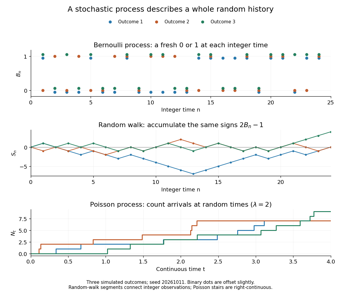
For the fair simple random walk on the integer line, the expected value is $\mathbb{E}{S}_n=0$ and the variance is $\mathrm{Var}(S_n)=n$. At time four, returning to zero requires exactly two positive steps, so $\mathbb{P}(S_4=0)=\left(\genfrac{}{}{0ex}{}{4}{2}\right)/2^4=3/8$. A rate-two Poisson process instead has $\mathbb{P}(N_1=0)=e^{-2}\approx 0.1353$. A single realized sample path does not establish either probability: they follow from the specified joint probability distributions.

The most revealing feature is often dependence. Two stochastic processes can have identical marginal distributions at every time while one forgets everything at the next step and the other repeats its first value forever. Their finite-dimensional distributions and covariance functions distinguish them. That extra structure is what makes a stochastic process useful for prediction.

The total differential is the linear map that combines the first-order responses to simultaneous changes in all coordinates. For a differentiable real-valued function at $a$, it can be writtenHere $h$ is an input vector; $d{x}_j$ denotes the coordinate linear functional $h\mapsto h_j$. The coordinate formula and the Fréchet derivative describe the same linear map. The defining approximation isThe little o notation says the remaining approximation error becomes small relative to the input norm, across every direction of approach.^[ref]

For $f=x^2+xy+2y^2$ at $a=(1,1)$, $d{f}_a(h,k)=3h+5k$. A simultaneous change $(h,k)=(0.02,-0.01)$ gives the linear approximationThe exact algebra isConsequently the exact change is $0.0104$, and the approximation error is $0.0004$. If both input changes are halved, the linear prediction becomes $0.005$ and the error becomes $0.0001$: the first-order response halves, while the quadratic error falls by a factor of four. The right panel under directional derivative displays this comparison as the displacement is scaled.

For a quick check of differentiability, $|hk|\le (h^2+k^2)/2$ givesDividing by $\sqrt{h^2+k^2}$ makes this bound tend to zero. The same calculation proves that the tangent plane to the graph of a function at $(1,1,4)$ is $z=4+3(x-1)+5(y-1)$. It approximates the entire local surface, rather than only two coordinate slices.

The total differential is useful for estimating the combined effect of small input changes without reevaluating a complicated function. For example, if $|h|\le 0.02$ and $|k|\le 0.01$, then $|d{f}_a(h,k)|\le 0.11$. The exact remainder bound from the displayed polynomial is at most $0.0008$, so this example has $|\Delta f|\le 0.1108$ throughout that input rectangle. These are deterministic bounds; a variance calculation additionally needs a joint probability distribution and its covariances. A first-order estimate is also local: large changes require control of the remainder, not merely knowledge of the partial derivatives at one point.