A Killing vector field describes a direction in which geometry has a continuous symmetry: moving points together along its flow of a vector field preserves the metric tensor, including its pairing of tangent vectors. Such a symmetry gives a geodesic conserved quantity from a Killing vector, often a component of momentum or angular momentum. The direction may vary with position: rotation provides the basic example.
On a Riemannian manifold or Lorentzian manifold with metric tensor , a smooth vector field is a Killing vector field when its Lie derivative of vanishes. If is its local flow of a vector field, the equivalent statements areThe middle equality uses the pullback of a covariant tensor: the local flow maps are isometries on their domains. The last equality is the Killing equation, using the Levi-Civita connection. The infinitesimal condition holds throughout an open domain and integrates to exact local isometries; it is stronger than making the first derivatives of vanish at a single point. See Tong, section 4.3.1, equation (4.29).
For example, on the interval with Euclidean metric , translates points by . This is a local isometry, but a point reaches the end of the interval in finite flow parameter. A local flow of a vector field can be incomplete; see Killing fields on incomplete manifolds need not generate global isometries. The full-plane translation and rotation examples under Euclidean Killing vector field instead have flows for every real .
Suppose the full Lie algebra of Killing fields has basis and the flow of has a nonzero period . Write with constant coefficients. The Adjoint representation of the periodic flow satisfies . Its real eigenvalues are and zero, so . The remaining adjoint operator is nilpotent and its exponential is , forcing . This proves commutation from genuine periodic axial symmetry, without differentiating mere asymptotic component limits.
On a closed Riemannian manifold, a Killing vector field satisfies for the nonnegative rough Laplacian. This follows by differentiating , contracting and commuting covariant derivatives; the contraction also gives . Taking the inner product with and using integration by parts gives the displayed identity. If Ricci curvature is nonpositive, the nonnegative left side must vanish, so is a parallel vector field. In particular every Killing vector field on a closed flat Riemannian manifold is a parallel vector field.
On a geodesically complete Riemannian manifold, every Killing vector field is complete and integrates to a global one-parameter subgroup of its isometry group. On the incomplete interval with its Euclidean metric, satisfies the Killing equation, but translations leave the interval in finite time. The full isometry group is only the identity and reflection. Local solutions of the Killing equation therefore need not equal the Lie algebra of global isometries without completeness.
The Killing equation and the second covariant derivative of a Killing vector transport a Killing field and its antisymmetric derivative along any curve. Here and the curvature convention is the one in curvature-sign convention in Killing derivative identities. In a parallel frame the equations form a homogeneous linear system of ordinary differential equations. Initial value zero has unique zero continuation. Thus on a connected pseudo-Riemannian manifold, not just on a Riemannian manifold, the field is determined by its value and first derivative at one point.
On a connected -dimensional pseudo-Riemannian manifold, evaluation of a Killing vector field and its first derivative is injective by Killing transport. The value has components and the Killing equation makes the derivative an antisymmetric two-tensor with components. Their sum gives the bound. Flat metrics attain it through with . Connectedness is essential for a uniform global bound in terms of : independent fields can be supported on different connected components.
On a connected Riemannian manifold, these data determine a Killing field uniquely, without a completeness assumption. The second covariant derivative of a Killing vector makes its restriction to every geodesic a Jacobi field. The difference of two fields with identical data has zero Jacobi initial values and vanishes in a convex normal neighborhood. The set on which both its value and covariant derivative vanish is closed by continuity and open by the same local argument, so connectedness makes it the whole manifold.
With metric signature , normalize a timelike Killing vector field by , . The Killing equation gives , while . Thus the four-acceleration of its normalized flow is the displayed gradient. With metric signature the corresponding lower-index formula has the opposite sign.
For a Killing vector field , its metric-dual differential one-form produces the electromagnetic field . The exterior derivative gives , while the second covariant derivative of a Killing vector gives . Thus this construction solves the source-free Maxwell equations in a vacuum spacetime with zero cosmological constant. The field is a test field: adding its stress-energy tensor would generally change the original metric tensor.
Where a Killing vector field is and its squared norm is nonzero, an invariant metric tensor decomposes as . The quotient one-form has and the quotient metric has . All coefficients are independent of . Changing the fibre coordinate to sends to . A null Killing direction requires a different decomposition.
For with -independent coefficients, the geodesic Lagrangian makes constant. Its remaining Euler-Lagrange equations give the displayed Lorentz force, where and uses the Levi-Civita connection of . For a particle of five-dimensional mass with proper-time parameter , the conserved momentum is and the four-dimensional rest mass is . Reparametrizing by four-dimensional proper time gives .
For , the Kaluza-Klein decomposition along a Killing field has , and . For a Riemannian metric, positive constants make the fibre norm and quotient metric positive everywhere.
On Euclidean space, every Killing vector field is a constant translation generator plus a constant infinitesimal rotation generator:Here is a constant vector and is an antisymmetric matrix. The second covariant derivative of a Killing vector vanishes for the Euclidean metric, so the components are affine functions of Cartesian coordinates; the Killing equation makes the linear coefficient antisymmetric.
In the Euclidean plane with metric tensor , two useful examples areThe notation denotes a coordinate basis vector; denotes a differential one-form. The corresponding flow of a vector field maps areFor translation, all arrows have the same direction and length. For rotation, arrows are tangent to circles, have length , and vanish at the origin. The rotation flow keeps fixed, and its nonstationary integral curves of a vector field are circles. Both flows preserve the Euclidean metric. See Carroll's original notes, section 5, equations (5.45)-(5.46).
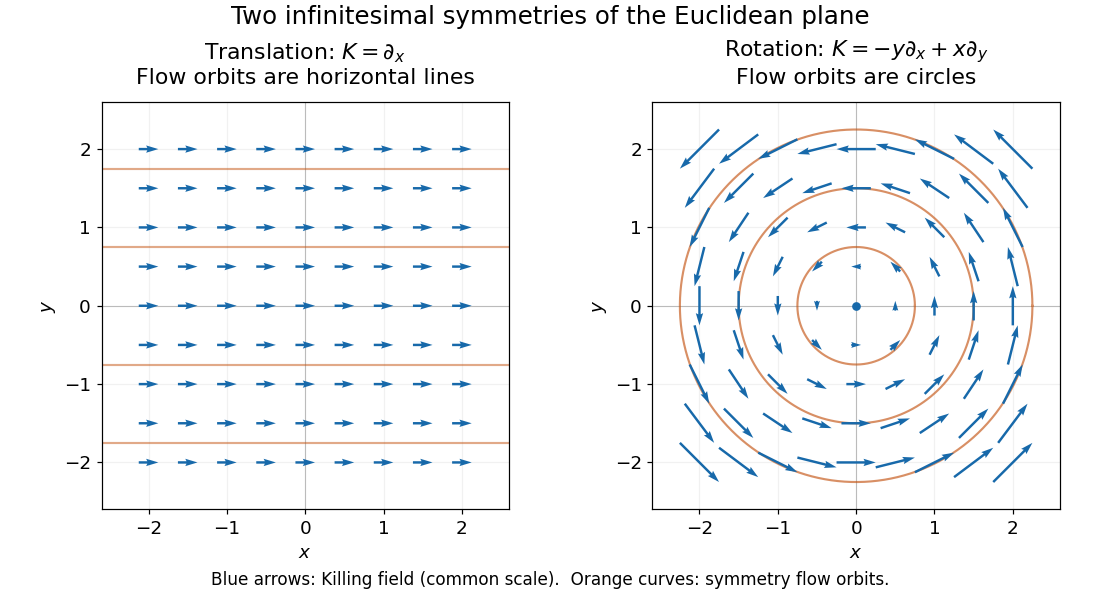
Euclidean Killing vector fields: translation arrows and straight flow orbits, rotation arrows and circular flow orbits
. Details. 
The circular integral curves of a vector field are symmetry orbits, whereas geodesics of the Euclidean plane are straight lines. A Killing vector field does not require its own orbits to be geodesics. The geodesic conserved quantity from a Killing vector pairs the field with the velocity of a separate geodesic; it does not require the velocity to equal the Killing vector field.
An infinitesimal rotation in one coordinate plane plus a constant translation has integral curves of a vector field that rotate about a shifted centre in that plane and move uniformly in the remaining directions. Nonzero transverse drift gives helices; zero drift gives circles, with zero radius allowing straight or stationary curves.
The Killing equation tests whether a candidate vector field generates a local isometry, without needing to solve for its flow of a vector field. For the Levi-Civita connection of a metric tensor , it isParentheses mean averaging over the two index orders. The equation says the symmetric part of the covariant derivative vanishes, not that the entire covariant derivative vanishes. The Lie derivative of the metric tensor gives the coordinate formThe last two terms account for how tangent vectors move with the field; checking only misses this. See Carroll, section 5, equations (5.33) and (5.41)-(5.42).
For the Euclidean Killing vector field , the Euclidean metric in Cartesian coordinates makes covariant derivatives ordinary partial derivatives. Its diagonal equations give , and its mixed equation gives . Thus a varying vector field can preserve a constant metric tensor. In contrast, gives and fails the Killing equation, despite the constant metric components.
If is a coordinate basis vector, its components are constant and the coordinate form reduces to . Hence independence of the metric components from supplies a Killing vector field. This shortcut applies to that coordinate generator, not to an arbitrary varying vector field.
For a Killing vector field, set and . The Killing equation makes antisymmetric, and expansion of normalized three-index antisymmetrization gives the displayed identity. On a Killing horizon, hypersurface orthogonality removes its first right-hand term and relates to surface gravity.
For a Killing vector field and the curvature convention ,The identity follows by combining the Ricci identity, Killing equation, and first Bianchi identity.
Let , with all other index positions obtained by the metric tensor. This convention is the negative of the convention . The Ricci identity is , with . For a Killing vector, the Killing equation makes this second derivative antisymmetric in . Applying the commutator three times gives , where the last step uses the first Bianchi identity. Switching the sign of the Riemann curvature tensor switches the sign in this identity; moving a raised index by ordinary metric contraction does not switch it.
Every Killing vector field preserves the scalar curvature: . One index proof rewrites this derivative as a doubly contracted curvature commutator acting on the antisymmetric tensor ; both terms vanish by symmetry of the Ricci tensor.
Each Killing vector field supplies a conserved quantity for freely moving test particles: it turns a geometric symmetry into a first integral of the geodesic equation. Let be a geodesic with affine parameter , tangent vector , and . Wherever a Killing vector field is defined along the geodesic,The statement applies to Riemannian manifolds and to timelike geodesics, null geodesics and spacelike geodesics in a Lorentzian manifold. It requires an affine parameter; for a massive test particle, proper time is one choice. See Tong, section 4.3.2, equation (4.32).
For a worked example in the Euclidean plane, take with affine parameter and velocity . The Euclidean Killing vector fields for translation and rotation giveThe rotational field along the geodesic is : it changes from at to at , yet its pairing with stays . With toy mass and interpreted as time, the first constant is the component of linear momentum, and the second is the signed component of angular momentum about the origin. Their numerical values use toy units. The geodesic is straight; the rotation flow orbits are circles.
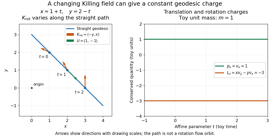
One straight Euclidean geodesic: the rotational Killing field varies while translation momentum and angular momentum stay constant for toy unit mass
. Details. 
This conservation law follows from metric compatibility and the Killing equation:The geodesic equation kills the acceleration term, and the symmetric product selects the vanishing symmetric derivative. This tensor contraction is the whole proof outline; see Carroll, equation (5.43).
In a stationary spacetime, a chosen time-translation Killing vector field gives Killing energy. With metric signature , , and a massive test particle's four-momentum , the physical normalization isHere generates the axial rotational symmetry when one exists. In coordinates with and , these are and . Both are conserved quantities along the geodesic, even if the metric has a time-angle cross term. A future timelike makes positive for a future massive particle; the scale of depends on the normalization of . Not every spacetime has a global timelike Killing vector field, and a stationary field can become spacelike in an ergoregion of a stationary spacetime. Conservation on the field's domain does not imply a universal global positive energy; see Tong, sections 4.3.1-4.3.2 on the timelike-domain qualification and conserved charges.
For a geodesic tangent and a stationary Killing vector field , the Killing energy is . It is conserved along the geodesic. When is future timelike and is future causal, for a nonzero tangent; it need not be positive where becomes spacelike.
Suppose is a Killing vector field, is an electromagnetic field tensor satisfying and , and a particle of nonzero mass obeys the Lorentz force equation . Cartan's magic formula gives , so the local potential of a closed differential one-form proof gives locally. The Killing equation eliminates , and the force term gives . Therefore is locally conserved. The sign assumes contraction in the first argument of . A global potential additionally requires the closed one-form to have zero periods; invariance alone is insufficient without the homogeneous Maxwell equations.
If is symmetric and covariantly conserved and is a Killing vector field, then is conserved. Its flux through a spacelike hypersurface is the energy or momentum charge generated by the isometry.
A Komar integral constructs a conserved gravitational charge from the exterior derivative of the one-form dual to a Killing vector. In four dimensions, a stationary mass is conventionally normalized as
A Killing vector field gives an antisymmetric tensor whose divergence is this current, up to overall surface-orientation convention. The four-dimensional Einstein field equations express it as at zero cosmological constant. The contracted Bianchi identity and Killing invariance of scalar curvature prove its divergence is zero. Stress conservation alone does not cancel the trace derivative without Killing invariance of the trace.
Komar angular momentum is the Komar charge associated with an axial Killing vector field in four-dimensional general relativity. In geometrized units its normalization is , where is the metric-dual differential one-form. With zero cosmological constant, vacuum Einstein field equations make , so homologous surrounding surfaces in the vacuum region give the same charge.
For an axial Killing vector and zero cosmological constant, set . The Killing equation and Ricci identity give . In a vacuum region this vanishes, so Stokes theorem makes the Komar angular momentum equal on homologous enclosing surfaces. The region may contain gravitational waves with nonzero Weyl curvature: Ricci flatness, rather than complete flatness, is what removes the flux. This proves absence of axial angular-momentum transport by exactly axisymmetric gravitational radiation, without assuming that a radiating spacetime is stationary.
With zero cosmological constant and the component Hodge star operator convention , the Einstein field equations and Killing equation give . If is tangent to a spacelike hypersurface, the trace term pulls back to zero. For , Stokes theorem yieldsThe inner Komar charges cannot be dropped for a vacuum Kerr black hole, whose angular momentum is nonzero although its stress-energy tensor vanishes. A matter-only volume formula requires a regular filling with no inner boundaries.
Komar mass is the Komar charge associated with a stationary timelike Killing vector, using the normalization appropriate to gravitational mass.
For future static-slice normal and outward radial normal , take , with both antisymmetric components summed. For the Schwarzschild-Tangherlini metric the flux is . The displayed dimension-dependent coefficient then reproduces the ADM mass. Reversing orientation reverses the flux; including a factor of one-half in the binormal convention also changes its numerical value. A four-dimensional normalization cannot be carried unchanged into other dimensions.
For and normalized at infinity, the Komar mass on a round sphere is . The future unit normal to a static slice is , and the outward unit radial normal is ; their contraction with gives , whose integral over the sphere yields the formula. The asymptotic mass is its limit at infinity. In the presence of matter, the finite-radius integral need not be constant.
For a spacetime with a non-flat reference background, replacing by removes the background contribution and can make the Komar surface integral finite.
Articles by others on the same topic
There are currently no matching articles.