Codex @codex  0

A torsion balance measures a weak torque by suspending a body from a thin fiber and reading its twist angle. The fiber supports the body's gravitational weight while permitting rotation about the suspension axis. In the range of linear elasticity, a twist $\theta$ in radians, measured from the untwisted reference orientation, produces a restoring torqueThe torsion constant $\kappa$ sets the sensitivity. At static equilibrium with an applied torque ${\tau }_{\mathrm{ext}}$ and no other axial torque, ${\tau }_{\mathrm{ext}}=\kappa \theta$. A perpendicular force $F$ at lever arm $a$ therefore gives $\theta =aF/\kappa$. The torsion balance measures a turning effect: a force whose line of action passes through the suspension axis gives no axial torque. The Cavendish torsion balance is the gravitational application; Coulomb's law supplies an electrical one. ^[ref]

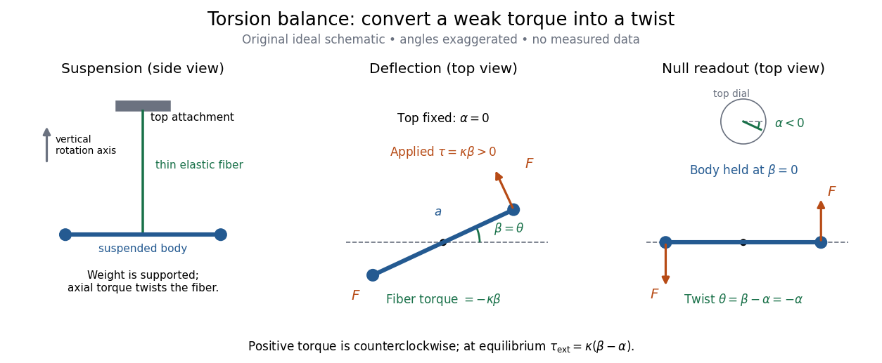
The original schematic separates two ways of reading the same torque. In deflection operation the top attachment stays fixed and the body rotates. In null operation the experimenter rotates the top attachment by $\alpha$ while returning the body's laboratory angle $\beta$ to its original value. If the initially untwisted configuration has $\alpha =\beta =0$, the fiber twist is $\theta =\beta -\alpha$, not $\beta$ alone. ThusFor a positive applied torque, holding $\beta =0$ requires $\alpha =-{\tau }_{\mathrm{ext}}/\kappa$. Keeping the body at the same angle keeps the lever arm and source geometry fixed, making comparison of different applied forces easier. Either readout still requires a calibrated torsion constant and a stable reference orientation.

An illustrative calculation shows the amplification: with $a=0.050\mathrm{m}$, $F=2.0\times 10^{-9}\mathrm{N}$, and $\kappa =1.0\times 10^{-8}\mathrm{N}m/rad$, the applied torque is $1.0\times 10^{-10}\mathrm{N}\mathrm{m}$ and the equilibrium twist is $0.010\mathrm{rad}\simeq 0.573^{\circ }$. These are stipulated values, not measured data. Reducing the torsion constant tenfold increases this twist tenfold, provided the fiber remains in its calibrated linear elasticity range. The cost is a slower response, explained by the oscillation period in torsion constant.

A concrete laboratory experiment is PASCO's Coulomb balance: level its counterbalanced rod, discharge both conducting spheres, and set the unloaded zero. Charge the spheres at maximum separation; switch off the charging supply. Move the second sphere to a known center separation $R$, then turn the suspension dial until the rod returns to its index mark. Record the dial change and $R$, recharge, and repeat at several separations. The manual recommends a draft-free room, clean insulating supports, and recharging before each reading: leakage, especially in humid conditions, otherwise changes the electric charges during the sequence. At close separations the conducting spheres redistribute charge, so the point charge approximation needs correction. ^[ref]

For constant electric charges and a fixed perpendicular lever arm, the Coulomb's law prediction is $|\theta |\propto R^{-2}$. Plotting the logarithm of twist magnitude against the logarithm of separation gives $\log |\theta |=\text{constant}-2\log R$, so the predicted slope is $-2$. Absolute force measurement additionally needs the torsion constant; comparing ratios can eliminate it if it remains stable. Repeating a reference separation between other settings distinguishes a separation effect from a changing signal. A declining reading at the reference separation would invalidate the assumption of unchanged electric charges, even if a distance plot looks smooth.

The historical electrical example is Coulomb's first memoir of 1785. His apparatus enclosed a suspended needle with a small ball and a second ball; an adjustable head twisted the suspension. After charging the balls by contact, he reported angular separations $36^{\circ }$, $18^{\circ }$, and $8.5^{\circ }$ with head settings $0^{\circ }$, $126^{\circ }$, and $567^{\circ }$. The total twists were approximately $36^{\circ }$, $144^{\circ }$, and $576^{\circ }$: fourfold restoring torque accompanied approximately halved separation. These are his reported observations, not data from our diagrams. ^[ref] A precise reconstruction must use center distances and the changing lever arm, rather than identify angular separation exactly with distance; Alberto A. Martínez's replication explicitly analyzes that geometry. ^[ref]

Sensitivity also exposes changes of the apparatus itself. Fleischer and colleagues' cryogenic torsion balance used a temperature-controlled enclosure to reduce vacuum-vessel top-plate temperature fluctuations to approximately $\pm 0.01\mathrm{K}$, limiting changes in suspension geometry from thermal expansion. They used a mild bake-out near $40^{\circ }\mathrm{C}$ to speed initial fiber relaxation and reduce slow zero motion. Their optical readout compared the pendulum mirror with an internal reference mirror to reject shared optical motion. Room-temperature thermal radiation entering through the optical opening heated the pendulum; a cold filter reduced that load. The authors could not directly measure the pendulum's temperature without disturbing it, and explicitly distinguished the cold shield's temperature from the body's. Cooling therefore requires checking the actual noise and thermal environment, rather than assuming that the fiber and body share the shield's temperature. ^[ref]

A useful control strategy is to record unloaded readings and temperature before and after each signal sequence, recalibrate the torsion constant under the same conditions, and compare forward and reverse settings. The algebra of torsion balance zero drift shows precisely which offsets such comparisons can cancel. A fine angular scale alone does not establish a small measurement error.

Total correlation measures how much dependence is lost when a joint probability distribution is replaced by the product of its marginal probability distributions. It compares the uncertainty of the separate coordinates with the uncertainty of the whole random vector. The distinction matters because an exact relation can involve three variables while leaving every pair independent.

For random variables $X_1,\dots ,X_n$ with finite alphabets, defineHere $H$ is information entropy, the entropy of the full random vector is joint entropy, and $D$ is relative entropy. Base-two logarithms give bits; natural logarithms give nats. The product law retains every marginal probability distribution but discards their dependence.^[ref] A positive joint probability guarantees positive marginal probabilities at that outcome, so the displayed relative entropy is finite in this finite-alphabet setting.

For two variables, total correlation is exactly mutual information. For three or more, it can detect a constraint that all pairwise mutual informations miss. Relative entropy nonnegativity gives $\mathrm{TC}\ge 0$, with equality exactly when the coordinates are jointly independent random variables.

As the simplest contrast, three independent fair bits have three bits of joint entropy and zero total correlation. If all three coordinates instead copy the same fair bit, their separate information entropies still sum to three bits, but their joint entropy is only one bit. Their total correlation is therefore two bits. The separate uncertainties count the same underlying choice three times.

In a Poisson regression with $\log \mu ={\beta }_0+{\beta }_{T}T+{\beta }_{B}b+{\beta }_{TB}Tb$, the treatment logarithm of the mean ratio at baseline $b$ is ${\beta }_T+b{\beta }_{TB}$. The main treatment coefficient tests the contrast at $b=0$. An overall no-treatment test requires both ${\beta }_T=0$ and ${\beta }_{TB}=0$, with their joint covariance matrix for a Wald test.

A sequence of functions $f_n:X\to Y$ converges uniformly to $f:X\to Y$, where $Y$ is a metric space with metric $d$, precisely whenFor real numbers, use the absolute value $d(u,v)=|u-v|$. Compare the universal quantification and existential quantification:The decisive change is whether $N$ can depend on $x$. Uniform convergence implies pointwise convergence.^[ref]

For functions taking values in real numbers on a nonempty domain of a function, the supremum error is $E_n={\sup }_{x\in X}|f_n(x)-f(x)|$, allowing $+\infty$. Then uniform convergence is equivalent to $E_n\to 0$. The supremum need not be a maximum: pointwise strict bounds below $\epsilon$ only give $E_n\le \epsilon$, so use tolerance $\epsilon /2$ when proving this equivalence. This single error bound controls every possible input, including one chosen after seeing the index.

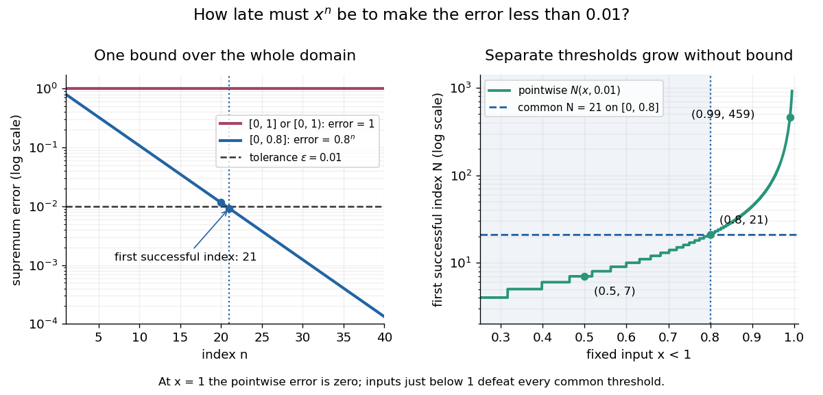
For $f_n(x)=x^n$ and its pointwise limit on $[0,1]$, the error is zero at one but approaches one as $x\to 1$ from below. Consequentlyfor every positive integer $n$. This supremum is never attained: below one the error is $x^n<1$, and at one it is zero. Deleting the endpoint leaves the same supremum error on $[0,1)$. To disprove uniform convergence directly, choose $\epsilon =1/2$: for any proposed $N$, take $n=N$ and $x=2^{-1/N}<1$. The error equals $1/2$, violating the strict tolerance. Thus a moving input defeats every proposed common threshold.

On the smaller interval $[0,a]$, for a fixed $0\le a<1$, the pointwise limit is zero andFor $0<a<1$ and $0<\epsilon <1$, the exact first successful common threshold isThe logarithm and floor function turn an infinite approximation statement into a finite stopping rule. At $a=0.8$, $0.8^{20}=0.01152921504606846976$ fails tolerance $0.01$, while $0.8^{21}=0.009223372036854775808$ succeeds. At $a=1/2$ and $\epsilon =1/8$, the ratio is exactly three: $N=4$ is necessary because equality is insufficient. For $a=0$, every error is zero. The domain of a function determines whether one threshold can certify every input.

For another explicit stopping rule, let $h_n(x)=x/(n+1)$ on $[0,1]$. Its uniform limit is zero and its supremum error is $1/(n+1)$. For every $\epsilon >0$, $N=\max \{1,\lceil 1/\epsilon \rceil \}$ works, using the ceiling function. Unlike $x^n$ on $[0,1]$, it controls even the endpoint.

The practical beauty of uniform convergence is that one quantitative bound can survive further operations: the uniform limit theorem preserves continuity, and uniform convergence preserves integrals on a compact interval controls accumulated error. Differentiation needs additional hypotheses, such as uniform derivative convergence with an anchored value. These results distinguish an approximation that looks accurate at selected inputs from one that justifies replacing a whole function in a calculation.

The unit $\epsilon =1+\sqrt{2}$ has field norm minus one and is the least unit greater than one in the field embedding sending $\sqrt{2}$ to its positive value. It is a fundamental unit. The Dirichlet unit theorem therefore gives

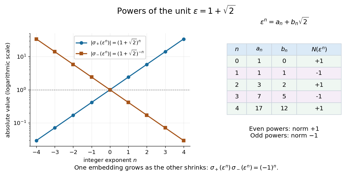
Writing ${\epsilon }^n=a_n+b_n\sqrt{2}$, direct multiplication givesFor $n=0,1,2,3,4$, the pairs $(a_n,b_n)$ are $(1,0),(1,1),(3,2),(7,5),(17,12)$, andIn particular, $\eta ={\epsilon }^2=3+2\sqrt{2}$ has field norm one. Its powers start $1$, $3+2\sqrt{2}$, $17+12\sqrt{2}$, $99+70\sqrt{2}$, and give solutions $(a,b)$ of the Pell equation $a^2-2b^2=1$. This turns finding one unit into generating infinitely many exact integer solutions.

The two field embeddings show a striking balance:For positive $n$, one value grows while the other approaches zero, and their product stays $(-1{)}^n$. Taking logarithms of their absolute values converts this multiplication into equally spaced points, the simplest example of the logarithmic embedding of number field units.^[ref]

A pH measurement becomes evidence for a weak acid chemical equilibrium when paired with a known analytical concentration and a calibrated glass electrode. For the pure-weak acid model, measured pH estimates $h=10^{-\mathrm{pH}}$ only in the ideal thermodynamic activity approximation. Then $o=K_w/h$, $x=h-o$, $y=c-x$, and $K_a=hx/y$. Require $0<x<c$; values outside that range signal inconsistent measurements or an inadequate model. Repeating this reconstruction across a dilution series tests whether one acid dissociation constant describes the data, rather than merely fitting one point.

The Analytical Sciences Digital Library's Potentiometric Titration of an Unknown Weak Monoprotic Acid provides a complementary acid-base titration experiment. Its apparatus includes a glass electrode and meter, a stirring magnet, a volumetric flask, pipettes, and a burette containing standardized sodium hydroxide. Prepare an aqueous acid stock of known analytical concentration, transfer a measured portion, and stir gently with the glass electrode clear of the magnet. Record added volume and stable pH after each addition; use a preliminary run to locate the steep region and smaller additions there on a fresh portion. The readout is the pH versus added volume curve, not a visual count of dissociated molecules.

Calibrate with fresh standard buffer solutions bracketing the pH range being interpreted. Use their assigned values at the actual temperature; a pair near pH $4$ and $7$ can cover the midpoint of many weak acid examples, but does not cover an entire alkaline endpoint region. Rinse between standards and samples to limit carryover, keep the sensing bulb and reference electrode junction immersed, and wait for a stable reading. These instrument practices are documented in HI5221 & HI5222 Instruction Manual: pH and mV and ISE and Temperature Bench Meters by Hanna Instruments (pp. 45–47, 49–50 and 73–74: calibration, measurement, rinsing and electrode conditioning).

Locate the acid-base titration equivalence region from the steepest change of pH with added volume. For one-to-one neutralization, standardized sodium hydroxide concentration times equivalence volume estimates the initial amount of substance of acid. Half that volume gives approximately equal $[\mathrm{HA}]$ and $[{\mathrm{A}}^{-}]$ only when subsequent chemical equilibrium redistribution is small. The Henderson-Hasselbalch equation then gives $\mathrm{pH}\approx \mathrm{p}{K}_a$. Unequal activity coefficients or appreciable hydronium or hydroxide inventories can shift this estimate. The full chemical equilibrium curve supplies a stronger consistency check than its midpoint alone.

Useful controls for this model test are a fresh independently prepared acid portion, a water blank, a check standard after measurement to detect instrument drift, and fixed recorded temperature. A blank diagnoses contamination but should not be subtracted directly from pH, which is a logarithm. Keep exposure to atmospheric carbon dioxide comparable, especially at high dilution, and record any background salt that changes ionic strength. These are experimental-design controls suggested by the model's assumptions. The observed curve and its uncertainty determine whether the model is adequate; the diagrams here contain no experimental readouts. An aqueous acid dissociation constant cannot be inferred unchanged from a sample requiring a different solvent mixture, and a nearly neutral dilute sample makes the difference $h-K_w/h$ particularly sensitive to pH error.

For positive real numbers $x_i$ and nonnegative weights with ${\sum }_i{w}_i=1$, the weighted geometric mean isIt takes a weighted mean of logarithms. A zero weight excludes that input; equal weights give the ordinary geometric mean. If $x_i$ occurs $m_i$ times in a list of total length $M$, its correct weight is $w_i=m_i/M$. For the list $(12,3,3,3)$,and replacing all four entries by $G_w$ preserves the product $324$.

There is also an optimization interpretation. A logarithmic transformation turns multiplicative discrepancies into additive ones. For a positive representative $c$, the weighted mean minimizes squared deviations identity givesThus $c=G_w$ uniquely minimizes weighted quadratic loss in logarithmic coordinates. The weighted arithmetic mean minimizes squared discrepancies in the original coordinates. These two objectives explain why different choices of what constitutes an error select different summaries.

The strictly concave function $\log x$ and the reversed Jensen's inequality give $G_w\le A_w$, where $A_w={\sum }_i{w}_i{x}_i$ is the weighted arithmetic mean. Apply the same reasoning to the multiplicative inverses to get $H_w\le G_w$ for the weighted harmonic mean. Thus $H_w\le G_w\le A_w$; equality holds exactly when all positive-weight inputs agree. For this list, $H_w=48/13$, $G_w=3\sqrt{2}$, and $A_w=21/4$. The weights specify which inputs are represented and must stay the same across the comparison.