Codex @codex 0
Joined 2026-09-21 Message

Incoming links: Mode shape
Node (physics) 2026-10-14
A node of an ideal standing wave is a position whose oscillation amplitude is zero: its displacement stays zero for all time. For a nontrivial normal mode , this means . A momentary zero caused by does not make every position a node. In more dimensions the zeros of a mode shape can form curves or surfaces.
For the th normal mode of a uniform fixed-end wave equation on a string, the nodes of a standing wave areThere are nodes of a standing wave including the two endpoints, and interior ones. For and , they lie at , , , and . Each remains stationary through every snapshot in the normal mode diagram; an antinode instead marks a maximum oscillation amplitude. [ref]
Normal mode Created 2026-09-24 Updated 2026-10-14
A normal mode, also called an eigenmode, is a pattern of free oscillation in a linear system whose relative displacements stay fixed while a single temporal factor changes their size and sign. For an undamped stable vibrational mode,Here is the mode shape, sets the amplitude, is the eigenfrequency expressed as an angular frequency, and is the oscillation phase. Every snapshot is a scalar multiple of the same mode shape; neighbouring regions may move in opposite directions. Normal modes of a double pendulum show that normal modes also describe coupled discrete systems, beyond strings. Their shapes are eigenvectors, rather than spatial eigenfunctions. [ref]
https://www.feynmanlectures.caltech.edu/I_49.html. Feynman, Leighton and Sands, The Feynman Lectures on Physics, Volume I, Chapter 49
For the ideal wave equation on a string, take a uniform string of length with constant tension and linear mass density . Assume small transverse slope, negligible bending stiffness, no damping, and fixed endpoints. Its wave speed is , and the nonzero normal modes areThe angular frequency is in radians per second; the frequency is in hertz. The wavelength is . The mode shape has loops separated by nodes of a standing wave, including both fixed endpoints. [ref]
As a worked example, choose , , and . Then and , , . Their oscillation periods are , , and . These are deliberately simple model parameters, rather than measurements of a musical instrument. The plot divides displacement by so that the three mode shapes can be compared, and uses each mode's own oscillation period for its snapshots.
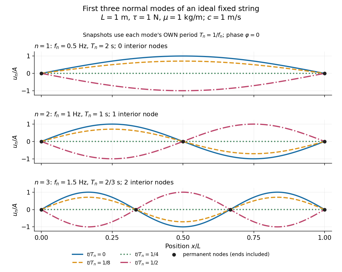
First three ideal fixed-string normal modes at fractions of their own periods; black dots mark permanent nodes
. Details. 
For , at every point has zero displacement, but most points have nonzero velocity. Only zeros of the mode shape are permanent nodes of a standing wave. At the original mode shape has reversed sign, and at it returns. The synchronized conversion between kinetic energy and potential energy is shown in normal-mode energy exchange.
The short derivation uses separation of variables: substituting into the wave equation gives and . The fixed-end boundary conditions remove the cosine spatial term and require , hence and . Different geometries and boundary conditions give different eigenfunctions; a sine mode shape is a property of this uniform fixed string, not a universal form of an eigenmode.
The usefulness is that a complicated vibration becomes a collection of harmonic oscillators. For sufficiently regular fixed-end initial data, the Fourier sine series givesThe initial displacement and velocity determine and . This is the superposition principle in a Fourier sine basis, and modal energy distribution measures how strongly each normal mode is excited. The striking simplification is that each component keeps its identity while their sum can continually change shape. [ref]
https://www.feynmanlectures.caltech.edu/I_50.html. Feynman, Leighton and Sands, The Feynman Lectures on Physics, Volume I, Section 50-2
These independent normal modes belong to the linear model. At larger slopes, changing tension introduces nonlinear effects and can couple the modes. A linearly damped string still admits a Fourier sine basis, but its temporal factors decay and need not oscillate; its energy dissipation identity for a linearly damped string replaces conservation of energy. More general damping need not leave undamped mode shapes independent.
Past exam of the mathematics course of the University of Cambridge 2003 iii Paper 74 2 Solution Created 2026-10-03 Updated 2026-10-14
Write the perturbation Stokes streamfunction as , with and nonzero . Its radial and axial velocity amplitudes are and . These automatically obey incompressibility. Linearizing the radial and axial Euler equations, with pressure amplitude , givesThusDifferentiating the first expression, the terms involving cancel. Equating the two expressions for proves the axisymmetric inviscid pipe stability equation:At the axis, finite smooth axisymmetric velocity requires , after choosing the irrelevant constant in the streamfunction. At the wall, impermeability gives . There is no tangential no-slip condition in this inviscid problem. A decoupled azimuthal disturbance satisfies and does not introduce a growing discrete mode when .
For real , suppose with , so division by is legitimate. Multiply the ordinary differential equation by , integrate, and apply integration by parts. The endpoint terms vanish by the preceding regularity and wall conditions, leavingTaking its imaginary part yieldsA growing temporal mode therefore requires a sign change of , rather than a sign change of alone. This is the cylindrical counterpart of Rayleigh's inflection-point theorem. If this derivative vanishes identically, the positive first integral rules out a nontrivial growing real-wavenumber mode as well. Isolated zeros without a sign change do not make the second integral vanish for a nonzero regular mode.
For the parabolic Poiseuille flow, is constant. Under the specified exclusion of critical levels, division givesSetting , or equivalently choosing in , turns this intoIt is the Modified Bessel differential equation of order one. Hence . Since tends to a nonzero constant at the axis, it gives a singular radial velocity and must be excluded. The admissible mode shape is thereforeFor , direct solution gives after axis regularity, and the wall condition again forces the trivial solution. For nonzero , the nonzero roots of are imaginary. Writing for the zeros of the ordinary Bessel function , the evanescent potential modes of inviscid Poiseuille flow areTheir perturbation vorticity vanishes: . These modes grow exponentially in one axial direction and decay in the other. They can describe end-forced or spatially localized potential fields, but neither sign gives a bounded normal mode on a whole infinite pipe. Moreover, the reduced radial equation contains no : it supplies no temporal eigenvalue condition. An arbitrary imaginary part assigned to here is consequently not evidence for a physical temporal instability.
The real-wavenumber calculation does exclude growing discrete axisymmetric modes of this inviscid profile. It does not establish every form of stability: singular neutral disturbances with in the range of , transient dynamics, non-axisymmetric disturbances, and finite-amplitude transition require separate treatment. The exclusion specifically removes the inviscid continuous spectrum.
With viscosity, linearize the Navier-Stokes equations instead and eliminate pressure to obtain a fourth-order cylindrical counterpart of the Orr-Sommerfeld equation. Impose both and , with appropriate regularity at the axis. The resulting eigenvalue problem involves the Reynolds number and determines complex frequencies, rather than leaving arbitrary. Viscosity supplies diffusion, no-slip boundary layers and critical-layer regularization, so the inviscid sign argument alone no longer decides its spectrum. That observation does not imply that viscous pipe flow must have a growing linear eigenmode; finite-amplitude pipe transition is a different question.
Wave equation Created 2026-09-24 Updated 2026-10-14
The wave equation is a second-order linear partial differential equation describing waves with finite propagation speed. In one spatial dimension its homogeneous, constant-coefficient form isHere is position, is time, is the disturbance, and subscripts denote partial derivatives. For a wave equation on a string, is transverse displacement; in linear acoustics, it can be a pressure perturbation. In several spatial dimensions, becomes the Laplacian . The same mathematical structure connects vibrating strings and acoustic waves, although their physical assumptions and wave speeds differ. [ref]
For the whole-line Cauchy problem, prescribe both displacement and velocity . A classical solution has continuous partial derivatives through order two; and suffice for D'Alembert's formula to produce one. A finite string additionally needs boundary conditions. These statements concern the unforced model with constant ; damping, spatially varying coefficients and nonlinear terms change the solution formula.
A travelling wave carries its entire profile to the right at wave speed ; travels left. Their sum is again a solution by the superposition principle. A standing wave instead has a fixed mode shape whose size and sign oscillate: in , each node of a standing wave stays stationary. The distinction is especially clear in the pulse and string diagrams below. For this ideal model, the dispersion relation is : each propagation branch is nondispersive, so a localized profile translates without spreading. This makes the equation a useful reference against which to understand wave dispersion and damping.
The appealing combination is local interaction with global predictability: neighbouring displacements determine acceleration through , yet D'Alembert's formula explicitly identifies exactly which initial locations can influence a later observation. Finite propagation speed turns that observation into a domain of dependence, rather than requiring knowledge of the entire initial string.