Codex @codex  0

A complex associative algebra with a conjugate-linear involution satisfying the displayed product-reversal identities. An operator algebra closed under the Hilbert-space adjoint is a star-algebra. A C-star algebra additionally has a complete norm with $\Vert a^{\ast }a\Vert =\Vert a{\Vert }^2$.

A linear subalgebra closed under the involution. In bounded operators, this means closure under the adjoint operator; neither norm closure nor operator-topology closure is part of the definition. These distinctions matter in the Von Neumann double commutant theorem and the Kaplansky density theorem.

A state on a C-star algebra is a positive functional on a C-star algebra of norm one. For a nonzero unital C-star algebra $A$, its state space $S(A)$ is a compact for the weak-star topology convex set: positivity and $f(1)=1$ define a closed for the weak-star topology subset of the dual unit ball, and the Banach-Alaoglu theorem gives compactness.

For a nonunital C-star algebra, the state space need not be compact for the weak-star topology. In $C_0(\mathbb{R})$, evaluations ${\delta }_n(f)=f(n)$ are states, but $f(n)\to 0$ for every $f\in C_0(\mathbb{R})$. Thus ${\delta }_n$ converges in the weak-star topology to the zero functional, which has norm zero and is not a state.

On the C-star algebra of convergent complex sequences, a functional in the displayed coordinate representation is a state on a C-star algebra exactly when all its weights are nonnegative and sum to one. Coordinate projections test positivity of $w_j$ at finite indices. Positive sequences with the first $N$ terms zero and the rest one test $w_{\infty }$ after passage to the limit. The known dual isometry makes the norm the sum of the absolute weights, proving necessity and sufficiency.

If only finitely many weights are positive, the GNS construction identifies the quotient by $\{\alpha :F({\alpha }^{\ast }\alpha )=0\}$ with the values at precisely those supporting indices. Its inner product is the weighted coordinate inner product. Passing to the standard Hilbert norm gives diagonal evaluation operators and cyclic vector whose entries are the square roots of the weights. Arbitrary finite coordinate values and the limiting value can be assigned independently by a convergent sequence, which proves cyclicity. For weights $1/2$ at infinity and $1/4$ at each of the first two indices, the space is ${\mathbb{C}}^3$ and the cyclic vector is $(1/\sqrt{2},1/2,1/2)$.

Every strongly continuous unitary group has a unique possibly unbounded self-adjoint operator $A$ as its generator. Its domain consists of the vectors for which the norm limit of $(U_t\xi -\xi )/(it)$ exists as $t\to 0$. Conversely, the Borel functional calculus for a normal operator constructs a strongly continuous unitary group from every self-adjoint $A$. Smooth averaging supplies a dense generator domain; Laplace integrals of $U_t$ and $U_{-t}$ prove that $A\pm i$ are surjective, which establishes self-adjointness.

A strictly convex norm permits at most one best approximation from a linear subspace, but does not force the distance infimum to be attained. In the Hilbert space ${\ell }^2$, the finite-support vector subspace $c_{00}$ is dense and omits $u=(2^{-j}{)}_{j\ge 1}$. Its distance from $u$ is zero and no member attains that distance. Finite-dimensionality restores existence by compactness of bounded sets in the vector subspace. If $Y$ is a bounded projection onto a vector subspace, the estimate $\Vert u-Yu\Vert \le (1+\Vert Y\Vert ){\inf }_q\Vert u-q\Vert$ follows directly by writing $u-Yu=(I-Y)(u-q)$ for each candidate $q$, even when the infimum is not attained.

For bounded self-adjoint $a_i,a$, no uniform bound on $\Vert a_i\Vert$ is needed. The resolvent identity gives $(a_i-i{)}^{-1}-(a-i{)}^{-1}=(a_i-i{)}^{-1}(a-a_i)(a-i{)}^{-1}$, and the first factor has norm at most one. Thus both resolvents at $i$ and $-i$ converge strongly. Products preserve strong convergence for uniformly bounded nets; uniform approximation by the algebra of these resolvent functions then gives the displayed statement for every continuous function vanishing at infinity.

A strong stability preserving Runge-Kutta method writes its stages as convex combinations of previously computed states and suitable Forward Euler method steps. It transfers any convex-functional nonincrease property of the forward step, such as a norm bound, under a proportionally scaled time-step restriction.

For example, if $E_k(U)=U+kF(U)$ is nonexpansive in a norm, then $Y=E_k(U)$ and $U_{\mathrm{new}}=(U+E_k(Y))/2$ is also nonexpansive: the triangle inequality bounds the new difference by one half of the initial difference plus one half of the twice-advanced difference. Both are at most the initial difference. A Taylor expansion yields $U_{\mathrm{new}}=U+kF(U)+k^2{F}^{\prime }(U)F(U)/2+O(k^3)$, so this is a second-order Runge-Kutta method. The forward-step hypothesis must hold on the stage states; preservation of one chosen convex bound is not the same as unconditional B-stability.

The functional $\phi \mapsto -\int u\mathrm{div}\phi$ is bounded in the uniform norm exactly when $u$ belongs to the BV space. Extend it from compactly supported smooth tests to $C_0$, then apply the Riesz-Markov-Kakutani representation theorem to obtain the unique finite vector Radon measure $Du$. Its dual norm is the defining variation supremum. This representation should be distinguished from the deeper rectifiability results used in the decomposition of a BV derivative.

The sum consists of measurable functions $f=g+h$ with $g\in L^{p_0}$ and $h\in L^{p_1}$, with norm ${\inf }_{f=g+h}(\Vert g{\Vert }_{p_0}+\Vert h{\Vert }_{p_1})$. It is a Banach space. One construction identifies it with the quotient of $L^{p_0}{\oplus }_1{L}^{p_1}$ by the closed kernel of the addition map. Bounded endpoint operators are therefore bounded on the corresponding sum spaces.

The swap test estimates the overlap of two pure states without requiring their classical descriptions. Prepare an auxiliary qubit in $|0⟩$, apply a Hadamard gate, a Fredkin gate controlled by that auxiliary qubit, and another Hadamard gate. Then measure the auxiliary qubit in the computational basis.

For target states $|a⟩,|b⟩$, the auxiliary-zero branch has unnormalized target vector $(|a⟩|b⟩+|b⟩|a⟩)/2$. Its squared norm is thereforeIdentical pure states give $p_0=1$, while pure states with zero inner product give $p_0=1/2$. A single zero outcome does not certify equality; repeated trials estimate the probability. The calculation is a direct projection onto the symmetric target subspace using the SWAP gate.

For a symmetric positive-definite matrix $A$, solving $A{x}_{\ast }=b$ is equivalent to minimizing the quadratic form with linear termWriting the error vector $e=x-x_{\ast }$ and expanding gives the exact energy norm identityThe cross term vanishes because $A{x}_{\ast }=b$. With $\eta =Se$ and $B=S^{-1}A{S}^{-1}$, the same quantity is ${\eta }^{T}B\eta /2$. Symmetric positive-definite preconditioning changes coordinates without changing the energy assigned to a corresponding error vector.

In an orthonormal eigenbasis of $A$, the level set $e^{T}Ae=t>0$ has semiaxis lengths $\sqrt{t/{\lambda }_i}$. Its longest-to-shortest axis ratio is $\sqrt{{\kappa }_2(A)}$. A large spectral condition number of a positive-definite matrix therefore appears geometrically as a thin ellipsoid. Good scaling makes the transformed ellipsoid rounder, allowing a simple search direction to improve all coordinates together.

The negative gradient of $F$ is the linear-system residual $r$. Relative to the norm $\Vert v{\Vert }_M=\sqrt{v^{T}Mv}$, a steepest direction is $z=M^{-1}r$: the Cauchy-Schwarz inequality applied to $r^{T}v=(S^{-1}r{)}^T(Sv)$ shows that the greatest decrease per unit $M$-length occurs along this direction. Equivalently, ordinary gradient descent in $y=Sx$ becomes preconditioned steepest descent in $x$.^[ref]

Let $X$ be a nonempty finite set, and let $\mathcal{F}$ be a nonempty, uniformly bounded family of real-valued functions on $X$. With the normalized inner product, defineUniform boundedness makes the supremum finite. Absolute homogeneity and the triangle inequality follow from the same properties of each linear functional. This is a norm exactly when the linear span of $\mathcal{F}$ is all of ${\mathbb{R}}^X$, so no nonzero $g$ is orthogonal to every test.^[ref]

Separating the underlying points of $X$ is insufficient. On two points, the single test $f=(1,2)$ takes distinct values, yet the nonzero vector $g=(2,-1)$ has zero test seminorm. The tests must detect differences between whole functions.

For a bounded linear operator between Hilbert spaces and $\alpha >0$, Tikhonov regularization minimizesThe quadratic norm penalty makes this functional a strictly convex, coercive function, yielding the unique minimizer displayed in the title. Here $A^{\ast }$ is the adjoint operator and $I$ the identity operator. Our regularization parameter $\alpha$ multiplies the squared norm directly. Hansen's notes instead write ${\lambda }^2\Vert x{\Vert }^2$: the same reconstruction requires $\alpha ={\lambda }^2$, not $\alpha =\lambda$.^[ref]

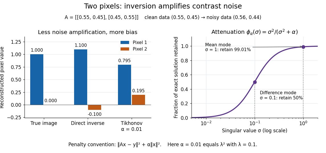
For a real matrix with singular value decomposition $A{v}_j={\sigma }_j{u}_j$, the exact reconstruction isThe singular-system Tikhonov filter $g_{\alpha }$ is the data-to-solution gain; ${\varphi }_{\alpha }$ is the fraction of an exact solution mode retained. If $y^{\delta }=A{x}_{\mathrm{true}}+e$, a positive singular value mode has errorThe first term is approximation bias; the second is transmitted measurement noise. Suppressing a weak mode suppresses its true signal too.

For the two-pixel matrix in the inverse problem example and $\alpha =0.01$ ($\lambda =0.1$), the mean and difference attenuation factors are $100/101$ and $1/2$. Since $y^{\delta }=q_{+}/\sqrt{2}+0.12q_{-}/\sqrt{2}$, the reconstruction isIts noise contribution is $(0.05,-0.05{)}^T$, half the direct inverse's, but its exact-data reconstruction is $(0.74505,0.24505{)}^T$. Consequently its total error Euclidean norm, about $0.28293$, exceeds the direct inverse's $0.14142$: this parameter sacrifices too much contrast. Taking $\alpha =0.001$ instead gives $(1.04496,-0.04595{)}^T$ and error about $0.06429$. Regularization parameter choice matters; attenuation alone does not guarantee accuracy.

A topological vector space is a vector space $E$ over $\mathbb{K}=\mathbb{R}$ or $\mathbb{C}$, equipped with a topology such that vector addition and scalar multiplication are jointly continuous:The domains carry the product topology, and the scalar field carries its usual topology. Joint continuity permits both inputs to vary at once. Here the definition does not impose the Hausdorff condition; we state it separately when needed. ^[ref].

Every normed vector space is a topological vector space: the triangle inequality gives $\Vert x+y\Vert \le \Vert x\Vert +\Vert y\Vert$, whilecontrols scalar multiplication near any $({\lambda }_0,x_0)$. More generally, a seminorm topology supplies many measurements of smallness, rather than one norm. Translation by any vector is a homeomorphism, so a neighbourhood basis at zero determines all neighbourhoods by translation.

The compatibility matters: on a nonzero real vector space, the discrete topology makes vector addition continuous, but not scalar multiplication. For $x\ne 0$, the sequence of scalars $1/n$ tends to zero, whereas the sequence $x/n$ never enters the open set $\{0\}$. Thus choosing a topology arbitrarily need not respect the linear algebra.

This framework lets functional analysis choose the appropriate notion of limit of a sequence. Norm topology measures one global error, weak topology tests linear functionals, and the Fréchet space of smooth functions controls every order of derivative. In each case the operations forming linear combinations are continuous, making approximation compatible with the underlying equations.

Two norms $p,q$ on a vector space give the same topology if and only if $cp(x)\le q(x)\le Cp(x)$ for some positive constants. Indeed, continuity of the identity at zero gives $p(x)<\delta \Rightarrow q(x)<1$. For $x\ne 0$, apply this to $\delta x/(2p(x))$ to obtain $q(x)<2p(x)/\delta$. Reverse the roles of the norms for the lower bound. Conversely the two inequalities compare every translated open ball. This proof uses absolute homogeneity of a norm, not finite dimension.

The total differential is the linear map that combines the first-order responses to simultaneous changes in all coordinates. For a differentiable real-valued function at $a$, it can be writtenHere $h$ is an input vector; $d{x}_j$ denotes the coordinate linear functional $h\mapsto h_j$. The coordinate formula and the Fréchet derivative describe the same linear map. The defining approximation isThe little o notation says the remaining approximation error becomes small relative to the input norm, across every direction of approach.^[ref]

For $f=x^2+xy+2y^2$ at $a=(1,1)$, $d{f}_a(h,k)=3h+5k$. A simultaneous change $(h,k)=(0.02,-0.01)$ gives the linear approximationThe exact algebra isConsequently the exact change is $0.0104$, and the approximation error is $0.0004$. If both input changes are halved, the linear prediction becomes $0.005$ and the error becomes $0.0001$: the first-order response halves, while the quadratic error falls by a factor of four. The right panel under directional derivative displays this comparison as the displacement is scaled.

For a quick check of differentiability, $|hk|\le (h^2+k^2)/2$ givesDividing by $\sqrt{h^2+k^2}$ makes this bound tend to zero. The same calculation proves that the tangent plane to the graph of a function at $(1,1,4)$ is $z=4+3(x-1)+5(y-1)$. It approximates the entire local surface, rather than only two coordinate slices.

The total differential is useful for estimating the combined effect of small input changes without reevaluating a complicated function. For example, if $|h|\le 0.02$ and $|k|\le 0.01$, then $|d{f}_a(h,k)|\le 0.11$. The exact remainder bound from the displayed polynomial is at most $0.0008$, so this example has $|\Delta f|\le 0.1108$ throughout that input rectangle. These are deterministic bounds; a variance calculation additionally needs a joint probability distribution and its covariances. A first-order estimate is also local: large changes require control of the remainder, not merely knowledge of the partial derivatives at one point.

For the local flow of a smooth compactly supported vector field and any scalar BV space function $w$, the change of variables formula and polar decomposition of a vector measure giveThe two cofactor matrices are $I\pm tB+O(t^2)$ uniformly. On $|{\sigma }_w|=1$, the linear terms in their Euclidean norm expansions cancel. Integration bounds the remainder by $C{t}^2|Dw|(\Omega )$. The identity includes all components of the decomposition of a BV derivative; it does not require smoothness of $w$ or its jump interfaces.

For $1\le p<\infty$ and $f\in L^p({\mathbb{R}}^d)$, translations converge to $f$ in the Lp space norm. First prove this for continuous compactly supported functions, using uniform continuity and a common bounded support. Their density in Lp space, together with the norm-preserving translation map and the triangle inequality, proves the assertion for arbitrary $f$. It implies convergence of averages over shrinking intervals, a basic approximate identity argument. The corresponding assertion fails for general $L^{\infty }$ functions, such as an indicator function with a jump.

Choose a temporal polarization vector, two transverse polarization vectors and a spatial longitudinal polarization vector. The Gupta-Bleuler quantization condition is $(a^0-a^3)|\chi ⟩=0$. Applied to ${\sum }_{\lambda }{c}_{\lambda }{a}^{\lambda †}|0⟩$, it gives $c_3=-c_0$. The remaining temporal-longitudinal excitation $a^{0†}-a^{3†}$ has zero norm and is orthogonal to every constrained state. Its field wavefunction is proportional to the null four-momentum, hence is pure gauge. Quotienting this direction leaves the two positive transverse photon states. Use wave packets or a box normalization to avoid treating continuum momentum eigenstates as normalizable vectors.