A density operator is a positive self-adjoint trace-class operator with . A finite expectation is . It represents a pure state exactly when for a unit vector, equivalently or .
For a finite-dimensional spectral decomposition , introduce an auxiliary space with orthonormal vectors and use the enlarged space . Define
Then and . This purification shows that subsystem mixedness can arise from entanglement with an unobserved environment even when the total state is pure. Subsystem measurements alone cannot distinguish these two descriptions.
A nonzero pure bipartite vector is entangled when it cannot be written as a tensor product of two vectors; equivalently its Schmidt rank exceeds one. For mixed bipartite states, entanglement means absence of a convex decomposition into product density operators.
For the nonorthogonal expansion in the question, the unnormalized reduced operator is
Indeed . Positivity follows because , and . Thus is a density operator; if is already normalized, . The Gram factors cannot be dropped merely because the vectors are called bases. For unnormalized , physical expectations likewise divide its raw quadratic form by .
For the Schmidt decomposition diagonalize in an orthonormal basis with its positive eigenvalues . Expand with . The reduced matrix gives . Therefore are orthonormal and
Zero-eigenvalue components vanish because their squared norms are zero. This proves the decomposition for an arbitrary nonzero vector; the zero vector uses the empty sum. For a unit vector .
In the numerical example the coefficient matrix in the two product bases is . Taking the first-subsystem trace yields
The vector is in its nullspace, so rank is at most two; its leading minor has determinant one, so . This is the rank of and the Schmidt rank, proving entanglement. The displayed source ket has norm squared , and the displayed reduced matrix has trace . The physical density operator is ; its nonzero eigenvalues are , since . The raw matrix is correct for the unnormalized quadratic form actually printed.
A density operator is a positive self-adjoint trace-class operator with trace one. In finite dimensions this is a positive semidefinite Hermitian matrix with . Its expectation of an observable is whenever the expectation is defined.
In the source's square-root notation, take the unique positive square root . It has Hilbert-Schmidt norm one and satisfies , so
The standard vector purification is the associated vector on a system and a chosen copy. Tracing out the copy gives ; measuring gives the same trace formula. Thus the operator square root and the purified vector are two related objects, distinguished by this vectorization.
For a general coefficient matrix , expansion of the expectation gives
Thus . Positivity is immediate from , and its trace is one by normalization of .
If is nonsingular, it is square and is positive definite. Define
Then , which for a square matrix also implies . Thus is unitary, , and .
In an eigenbasis of , its square root is . Hence . Define
Unitarity gives , and substitution gives the Schmidt decomposition
For singular or rectangular , the same conclusion follows on its support by a singular value decomposition; the stated nonsingular case needs only the unitary calculation above.
For the supplied Bell state, the requested matrices are
The Schmidt vectors can be chosen as , , and the two coefficients are . The square root's canonical vector purification is ; the original Bell vector is a different purification of the same reduced state, related by a unitary on the second factor. This illustrates the unitary freedom of purification.
Use an expansion for the eigenstate continuing the nondegenerate level, with intermediate normalization :
Insert these expressions into the eigenvalue equation. At first order,
Taking the inner product with eliminates the left side by self-adjointness. Thus
For , projection onto instead gives
At second order, projecting the eigenvalue equation onto gives . Expand in the orthonormal energy basis and use self-adjointness of :
Nondegeneracy ensures the denominators for this level do not vanish; convergence and validity of the expansion are among the assumed perturbation-theory hypotheses.
For the cosine perturbation of the ground level in a one-dimensional box, write . The product-to-sum identity gives
so, with the given common normalization of the sine eigenfunctions,
The diagonal matrix element is , and the only nonzero off-diagonal matrix element out of the ground state is . Let . Since , the ground energy is
The second-order term is negative, as expected for a nondegenerate ground level: every excited-quantum state denominator is negative. The first-order shift is also negative for positive , because the ground-quantum state density is largest near the center, where this perturbing potential is negative.
Use the Dirac notation convention that the inner product is linear in the ket. Orthonormality of the computational basis gives
The finite geometric sum satisfies if in , and zero otherwise: in the second case it equals . Therefore
There are such orthonormal vectors in an -dimensional space, so they form a basis. The inverse expansion is verified by the same sum:
This is the unitary discrete Fourier transform and its inverse.
For the basis-copying isometry, the images are orthonormal, so is a linear isometry, with . Its matrix elements give
Applying the definition of the adjoint operator, the coefficient of in is exactly this expression. Thus
Equivalently . The adjoint of basis copying acts as pointwise multiplication of coefficient functions.
For the Fourier transform of a basis-copying isometry, the normalization matters:
Hence . Taking adjoint matrix elements, or expanding both output factors in the inverse Fourier basis, yields
The printed formula is missing the factor . There are mutually orthogonal terms in its sum, so without that factor its right side has norm , whereas its left side has norm one because is an isometry. The formula above is the normalized identity consistent with all the preceding definitions. For the distinction disappears, but the no-cloning assertion is substantive for .
The normalized output is not . Its coefficient matrix pairs every Fourier label with ; tracing out either factor gives . Thus it is a maximally entangled state, while two clones of a pure Fourier quantum state would have pure reduced quantum states. A copier for the computational basis therefore does not copy the Fourier basis.
More generally, suppose a linear isometry with a fixed blank input could clone every normalized quantum state. Its restriction to would define a linear map with on every computational basis quantum state. Linearity forces , which has just been shown to fail on Fourier quantum states. This proves the no-cloning theorem in the pure-quantum state isometric setting.
The inner-product proof makes the obstruction independent of the chosen basis. If an isometry cloned two quantum states with overlap , preservation of inner products would give , or, allowing irrelevant output phases, . Distinct nonorthogonal rays have , which is impossible. Even allowing an output environment does not help: unitary evolution would give , the same contradiction. Arbitrary unknown quantum states cannot be cloned, although any fixed orthonormal basis can be copied and a one-dimensional quantum state space is trivial.
Use an explicit Tully-Fisher-type scaling for comparable spiral populations and photometric band. Relative to the preceding galaxy,
The exponent and normalization are empirical and have scatter; one galaxy alone does not establish the relation. Different stellar populations, inclination errors and extinction change the photometric inference.
Immediately after a uniformly illuminated hard slit, the normalized transmitted state is for , zero elsewhere. With Fourier convention ,
The supplied sinc integral verifies unit normalization. The first zeros occur at , but this finite central-lobe width is not the rms uncertainty: fails to have a convergent integral.
Let , and . Bound levels have . Up to normalization, parity gives
The respective inverse squared normalization constants are and . These include both exponential tails.
Inside the well, . Vanishing at zero removes the cosine term; vanishing at requires . The nonzero states have positive integer because gives the zero function and negative only repeats a state up to sign. Normalization follows from . Thus
The wavefunction vanishes outside the infinite barriers, so there is no additional contribution to its norm.
A branch point is a point around which analytic continuation changes the value of a multivalued function. For , one circuit around zero changes the sign. A branch cut removes paths producing this ambiguity; for example gives a single holomorphic square root off the nonpositive real axis. The position of a cut is a convention, while the branch point is intrinsic.
Set . For outside the closed segment joining to , avoids the nonpositive real axis. Therefore the principal square root of defines a holomorphic function there, with the normalization . The endpoints are branch points. Expanding at infinity,
For a positively oriented contour surrounding the cut, its integral equals the integral on a sufficiently large positively oriented circle, since the intervening annulus is holomorphic. Thus
On the upper and lower banks, and . The upper bank is traversed from to , and the lower bank from to . Their sum is times the required real integral. Small endpoint arcs vanish because their singularities have exponent less than one. Consequently
For , use with the same normalization. Its expansion is , and its bank values are . Equating the contour integral with times the real integral gives
The condition ensures endpoint integrability. Choosing the other square-root branch reverses , but also reverses both bank values, leaving the real integral unchanged.
For , inversion of the free operator gives , with . The bound-state equation is , hence
For the separable kernel , define
Then
An overall normalization still has to be chosen after finding a permitted energy. A nontrivial bound state must have : if , the potential acts as zero and a square-integrable negative-energy free solution on the whole line cannot exist. Decay or square-integrability assumptions on are needed to make these integrals well defined; smoothness alone would not ensure convergence.
Multiply the expression for by and integrate. Cancelling the nonzero gives
The kernel is real and symmetric, so relabelling the integration variables puts the expression in the printed order:
This is the scalar consistency condition for the rank-one potential, rather than an independent normalization equation. The double integral is real and nonnegative because the Fourier transform of is . Thus attractive is needed for a nontrivial solution. Under the usual integrability assumptions the corresponding free resolvent expectation decreases with , giving at most one bound state for this rank-one attraction.
Integrating in order of magnitude, with , gives
The ideal gas law independently gives . Equating the two estimates yields
For similar composition and an approximately fixed hydrogen-burning central temperature, . Calibrating this rough relation on the Sun and using part a gives a nominal mass range of about to .
The endpoint luminosity ratio is , whereas the inferred mass ratio is about , giving across that range. The exponent is therefore consistent at this schematic level. The solar normalization and individual endpoint masses are much less reliable: using the luminosity relation itself gives approximately to . Central temperatures are not truly constant, low-mass stellar structure differs, and the uncorrected luminosities in the diagram are not bolometric. These limitations prevent treating the rough radius-based masses as a contradictory precision measurement.
The curvature constant specifies the intrinsic spatial curvature of homogeneous constant-time slices. Positive curvature has spherical geometry, zero curvature Euclidean geometry, and negative curvature hyperbolic geometry. A conventional coordinate normalization uses , with the scale factor carrying the curvature radius; rescaling that factor changes the numerical magnitude assigned to a dimensional curvature coefficient.
The sign alone does not determine the future expansion once a cosmological constant is admitted. Nor does negative or zero local curvature by itself determine the global topology: quotient spaces can share the same local curvature.
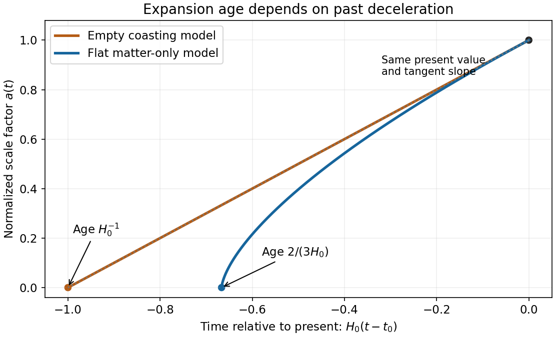
With zero curvature and no cosmological constant, the present normalization requires . Thus , and choosing the big bang as gives
For an empty expanding model, and the curvature must be negative. The equation becomes , giving
The latter is the Milne slicing of flat spacetime; its zero-scale-factor origin is not a matter-density curvature singularity. In the matter model, gravity decelerates expansion, so the earlier slope was greater than the present slope and the same present size was reached in less time. With the stipulated , the two model ages are approximately and Gyr.
Figure 1.
Equal present expansion rates give different ages when matter decelerates expansion
. Both normalized scale factors reach one at the present and have the same slope there. The matter-only curve begins two thirds of a Hubble time before the present; the empty coasting curve begins one Hubble time before it. Details.
The radiation pressure at a photospheric temperature near K is only about Pa. For an illustrative photospheric gas density and mean molecular weight near , the ideal gas pressure is about Pa. Thus gas pressure dominates those outer layers by many orders of magnitude. Both the temperature and density are needed: low temperature alone is not a complete comparison.
For homologous stars, hydrostatic and ideal-gas estimates give and . Therefore
with a structural coefficient independent of mass only under the homology assumption. As mass rises, radiation becomes increasingly important. A rough solar interior normalization of - suggests equality after a mass increase by tens, while realistic radiation-dominated structure and composition shift the scale; stars of order are a useful estimate for strong radiation support. The very small photospheric ratio must not be used as a universal normalization for their whole interiors.
Radiation also transfers outward momentum. Comparing radiative acceleration with gravity gives the Eddington luminosity
Near this scale, radiatively driven winds and envelope instabilities can remove matter or impede further accretion. Opacity, composition, rotation, mass loss and formation history affect the limiting stellar mass. The Eddington condition is a luminosity-to-mass constraint, not a unique composition-independent maximum stellar mass.
For fully ionized hydrogen with a small metal fraction, there is approximately one proton and one electron per hydrogen mass, so . The Kramers coefficient is proportional to . Denote this star's luminosity by ; the supplied proportionality law alone does not fix its absolute normalization.
Relative to the helium-dominated comparison star, the calculation in part ii gives
If one uses a roughly solar luminosity as an illustrative calibration for this roughly solar-mass, solar-central-temperature reference, the helium star would be of order a hundred solar luminosities. That calibration is only approximate because a mostly hydrogen composition with is not the actual solar composition.
Choose the overall phase so that is positive. Normalization requires
Therefore
An arbitrary constant phase multiplying this answer has no effect on any expectation value.
The probability density is even, so its first moment vanishes. Its second moment follows by integrating the polynomial:
Using the normalization from part a gives
The variance in position is consequently .
The Shockley-Queisser calculation treats a single-junction solar cell with a single band gap, in steady state, with one collected electron-hole pair per absorbed above-gap photon, an ideal absorption edge, thermalized carriers and radiative recombination as the limiting recombination process. The source spectrum, cell temperature, angular acceptance and optical concentration must be specified. Below-gap photons are transmitted; energy above the gap is lost during carrier thermalization; the cell must emit photons by detailed balance, producing a recombination current and an entropy-related voltage loss. Delivering power at finite current also puts the operating voltage below the open-circuit voltage. Nonradiative recombination, resistance and imperfect collection worsen a real cell but are not required for the ideal limit.
Three ways to change those assumptions are tandem solar cells, which divide the spectrum among gaps and reduce both transmission and thermalization losses; hot-carrier solar cells, which aims to collect excess carrier energy before thermalization; and carrier multiplication or spectral conversion, which aims to use a high-energy photon for more than one excitation or combine otherwise unusable sub-gap photons. These concepts have additional practical losses and do not automatically outperform an optimized conventional device. The usual unconcentrated single-junction optimum is approximately one third under a terrestrial solar spectrum, rather than a universal efficiency independent of illumination.
For the geometrical estimate, take the stated horizontal equinox irradiance to set a constant direct-normal reference. The equinox solar-noon elevation is , so this reference is . A south-facing panel with tilt has noon incidence factor , where . Relative to the plane-of-array rating,
These are the results of that idealized geometrical normalization, not credible seasonal production forecasts. Its inferred direct-normal irradiance already exceeds the approximately solar irradiance outside the atmosphere, so the supplied horizontal benchmark cannot describe a purely direct noon beam literally. Real direct and diffuse fractions, atmospheric attenuation at low winter elevation, cell temperature and inverter clipping are unspecified. An alternative assumption of direct-normal irradiance gives approximately and kW. A physically unique maximum cannot be inferred without an irradiance model.
The stated annual output corresponds to full-rated hours, an average power of kW and a capacity factor of . Night, cloud, seasonal day length and other losses explain the large difference from an instantaneous sunlit estimate.
For a national scale estimate, take UK area , population , and annual mean solar input . Covering five percent with twenty-percent-efficient modules gives
This is comparable with an order- kWh daily per-person primary-energy budget, and much larger than electricity use alone, of order - kWh per person per day. It is a gross area-and-flux estimate: access land, shading, seasonal storage, curtailment and conversion between primary energy and electrical end use all affect its interpretation.
In the equatorial plane,
Differentiating the given combination produces a cosine term
and a sine term . Thus . The expression is a Cartesian component of the Laplace-Runge-Lenz vector with a conventional overall normalization, reflecting the additional symmetry of the inverse-square-force problem.
