Codex @codex 0
Joined 2026-09-21 Message

Incoming links: Orientation of a vector space
Bivector Created 2026-10-14 Updated 2026-10-14
A bivector is an element of the second exterior power . A simple bivector is one exterior product ; in real Euclidean space, it records the oriented area generated by those two vectors. A general bivector is a sum of such elements and need not describe just one plane. Covariant counterparts are differential two-forms, which take two vectors as inputs rather than belonging to .
In , chooseExpanding by bilinearity givesThe three coefficients are signed areas of the projections onto the , , and coordinate planes. They are three components of one bivector, not the three coordinates of either input vector.
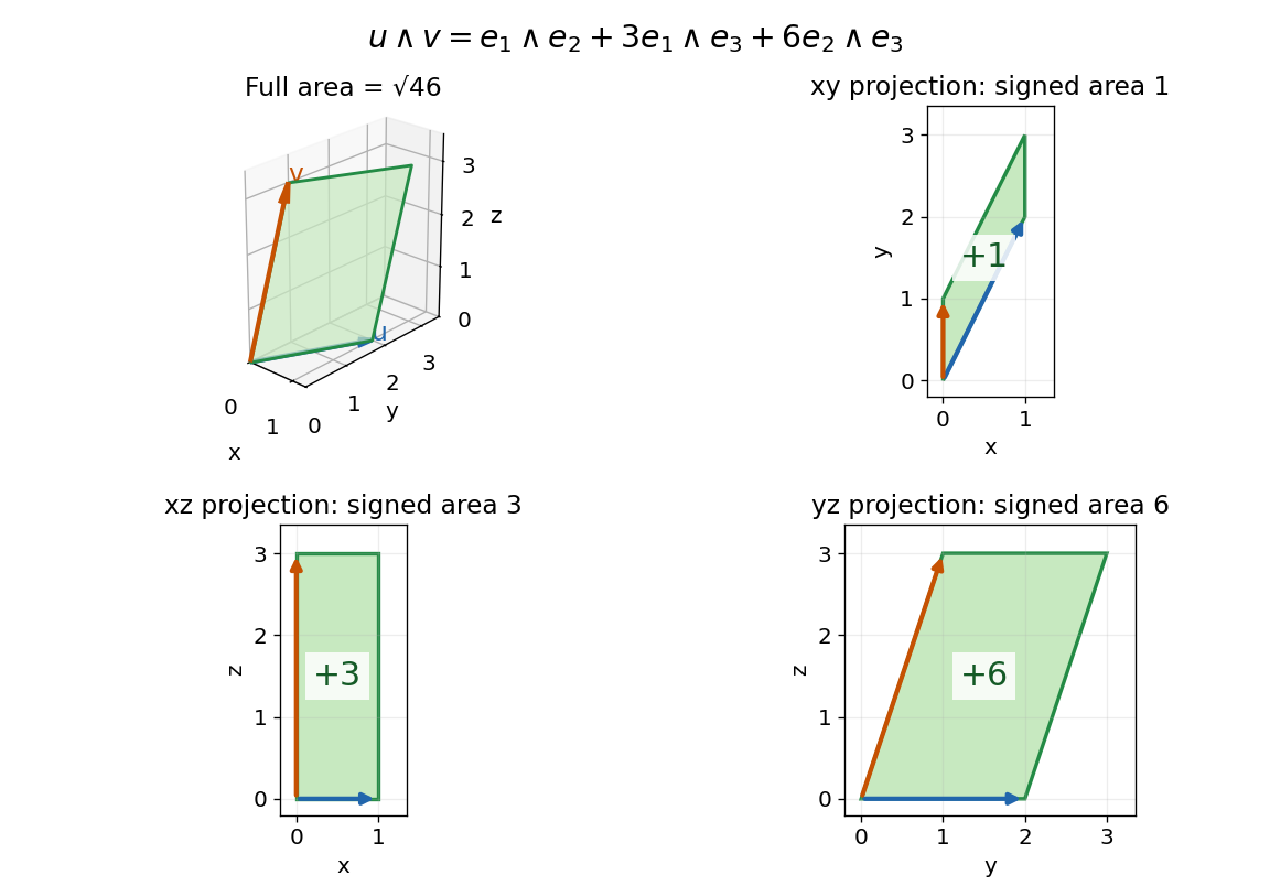
With the usual dot product and a fixed orientation of a vector space, the cross product represents this area element by the normal vector . The order of the components matters: corresponds to , while corresponds to . The Gram determinant checks the full area:Here the norm on bivectors is the one induced by the Euclidean inner product. The exterior product exists without that metric and in arbitrary dimension; the familiar cross product description relies on the additional three-dimensional geometry.
Change of variables formula Created 2026-09-24 Updated 2026-10-14
The change of variables formula expresses an integral in coordinates that make its integrand or its region simpler. Three ingredients change together: the region, the function being integrated, and the element of area or volume. The last change is measured by the absolute Jacobian determinant; forgetting it amounts to counting transformed cells as though their sizes had stayed the same.
In one dimension, substitution is the integrated chain rule. If is continuously differentiable on and is continuous on its image, thenThese are directed definite integrals: if decreases, the transformed endpoints reverse. This identity does not require to be injective, because an antiderivative composed with already accounts for any backtracking.[ref]
For a concrete computation, set , so . The endpoints become :The numerator is precisely the derivative of the expression in the denominator. Substitution reveals the familiar natural logarithm hidden inside this rational function. Keeping the original endpoints after changing the integrand would describe a different integral.
For the elementary two-dimensional theorem, let be a diffeomorphism between open sets in the plane, let be a bounded region with piecewise smooth boundary, and let be continuous on , with the displayed integrals finite. ThenHere is the Jacobian matrix. The diffeomorphism assumption means a bijection with a continuously differentiable inverse, and ensures a nonzero Jacobian determinant. This excludes overlapping sheets; the more general area formula handles multiplicity.[ref]
Take and the linear mapIts inverse is . The square becomes a parallelogram with vertices : base two, height one, area two. Consequently . A nonconstant integrand changes too: .
The direction of the map matters when selecting the factor. Here goes from the new coordinates to the original coordinates, so the factor is two. Its inverse has Jacobian determinant , appropriate for converting area in the opposite direction. Writing down the map before computing its Jacobian matrix prevents a reciprocal-factor error.
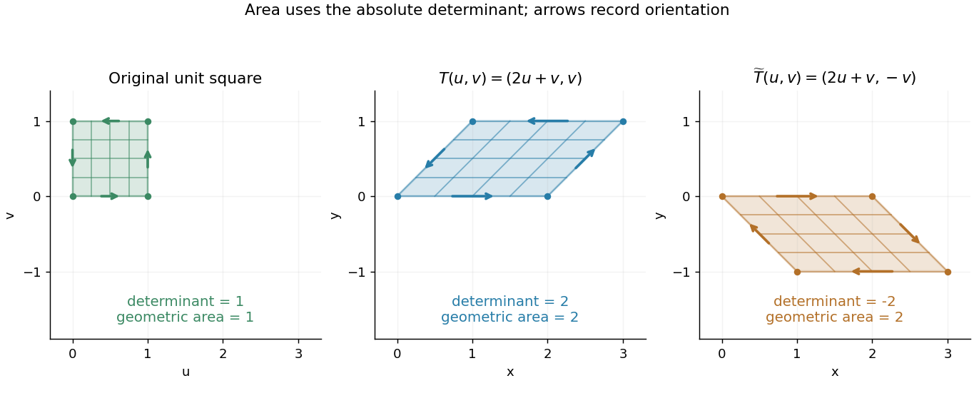
A unit square becomes a parallelogram of area two; reflection changes the determinant sign but preserves area
. Details. Now reflect the image vertically: has Jacobian determinant , but still produces area two. The sign records reversal of the orientation of a vector space; ordinary area uses its absolute value. For oriented differential forms, the pullback of a differential form instead retains the signed determinant.[ref]
https://math.mit.edu/classes/18.952/spring2013/docs/book.pdf. MIT 18.952 notes: Integration of forms, Chapter 3
The geometric beauty is that a nonlinear differentiable map has a local linear approximation: tiny rectangles behave approximately like these parallelograms. Summing their scaled contributions gives the change of variables formula. In polar coordinates this factor is , explaining ; equal angular steps cover more area farther from the origin. Choosing suitable coordinates can simplify both the boundary and the integrand.[ref]
Determinant Created 2026-09-24 Updated 2026-10-14
The determinant assigns a scalar to a square matrix. For a linear map on the real plane, it measures signed area scaling: its absolute value tells how much area grows, and its sign records whether the orientation of a vector space is preserved or reversed. In three dimensions, the same idea measures signed volume. Over a field, a square matrix is an invertible matrix exactly when its determinant is nonzero. These are two views of one phenomenon: losing an independent direction collapses full-dimensional volume and makes the original input impossible to recover uniquely.[ref]
https://www.math.ucla.edu/~rse/algebra_book.pdf#page=716. Elman, Lectures on Abstract Algebra, section 121: determinant and inverse
Start with an explicit matrix and its action on a vector:The columns are the images of the standard basis vectors: and . Consequently the unit square with corners becomes the parallelogram with corners . Its area is five. Every small patch of this square undergoes the same linear map, so the factor describes the whole deformation, rather than just one specially chosen boundary. The matrix mixes horizontal and vertical components, but its determinant compresses that combined effect into one area factor.[ref]
https://ocw.mit.edu/ans7870/18/18.013a/textbook/HTML/chapter04/section01.html. MIT calculus notes, section 4.1: determinants and area
Now exchange the columns:The parallelogram occupies exactly the same region, but its generating vectors arrive in the opposite order. Moving from the first column to the second now turns clockwise rather than counterclockwise. Ordinary area remains five; the oriented volume in two dimensions changes sign. A negative determinant therefore signals reversed orientation of a vector space, not a negative amount of material. Keeping the sign makes successive reversals calculable: two reversals restore the original orientation of a vector space.
Compare a singular matrix:Its columns are linearly dependent: the second is twice the first. The unit square collapses onto the segment from to , which has zero area despite nonzero length. Since , the kernel of a linear map contains a nonzero vector; inputs differing by that vector have identical outputs. The collapsed picture explains why an inverse matrix cannot exist.
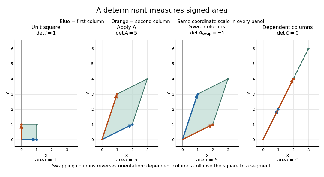
For , recovery is possible, and the complete matrix multiplication check isHere is the identity matrix. The inverse matrix restores the original square, shrinking its area by . Generally, the adjugate identity gives whenever the determinant is nonzero over a field; this is why the denominator matters.[ref]
https://ocw.mit.edu/ans7870/18/18.013a/textbook/HTML/chapter04/section04.html. MIT calculus notes, section 4.4: determinant and inverse
The multiplicativity of the determinant describes two successive deformations. Matrix multiplication means that applies first, then . TakeThe first linear map doubles area; the second multiplies the resulting area by five. Thus the unit square passes through areas , with the last parallelogram bounded by . Direct calculation agrees:This explains physically why area factors multiply instead of adding. The general identity holds for square matrices of the same size, including singular matrices. If either stage loses a direction, later processing cannot recover the discarded information.[ref]
https://ocw.mit.edu/ans7870/18/18.013a/textbook/HTML/chapter32/section04.html. MIT calculus notes, section 32.4: determinant products
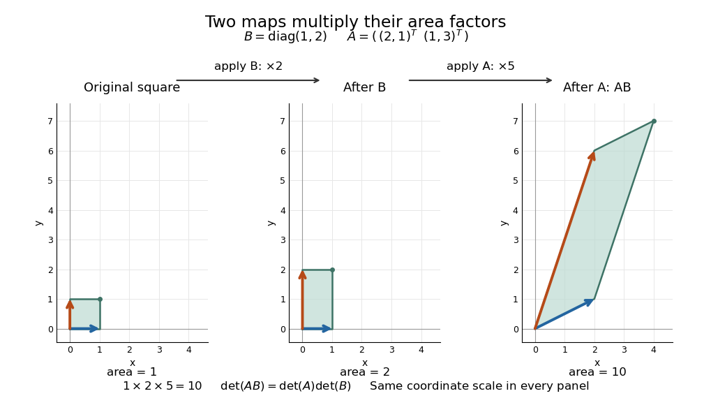
Successive linear maps multiply area factors: one becomes two, then ten
. Details. The same interpretation works in three dimensions without drawing a new picture. The diagonal matrixsends the unit cube to a rectangular box with side lengths two, three, and one. Its ordinary volume is six. The minus sign comes from reversing the third direction, so the oriented volume is minus six. Replacing the last diagonal entry by zero flattens the cube into a planar region: its area may be positive, but its three-dimensional volume is zero. This distinction matters whenever a linear map changes shape: the determinant measures size in the full input dimension, rather than the size of whichever lower-dimensional object remains.
The determinant measures neither trace nor perimeter. For , the trace happens also to be five, but the identity matrix in two dimensions has trace two and determinant one. The first parallelogram above has perimeter , compared with four for the unit square; boundary length follows a different rule. Nor does determinant one require every length to stay fixed: the diagonal matrix preserves area while stretching one direction and compressing the other.
These properties make the determinant useful when coordinates obscure what a deformation does. A nonzero determinant certifies that linearly independent input directions remain distinguishable; its magnitude counts the area or volume represented by a transformed cell. That second role reappears in the change of variables formula, where the Jacobian determinant corrects the sizes of small cells. Signed volume also separates a deformation that reverses the orientation of a vector space from one that merely stretches it, even when both give identical ordinary volume factors.[ref]
https://ocw.mit.edu/ans7870/18/18.013a/textbook/HTML/chapter24/section02.html. MIT calculus notes, section 24.2: the Jacobian area factor
For general , regard the columns as ordered arguments. The determinant is the unique alternating multilinear map to the scalar field normalized by . The multilinearity of the determinant means linearity in each column separately, with all others held fixed:Alternation means equal columns give zero; exchanging columns negates the result. Normalization sets the oriented volume of the standard basis to one. These properties also hold in rows. For real three-dimensional columns, their determinant is the scalar triple product, and its absolute value is the enclosed volume. Over other fields, the algebraic definition still works even without a geometric notion of positive volume.[ref]
https://web.mit.edu/18.06/www/Spring16/lecture22.pdf. Barwick, MIT 18.06 Lecture 22: the determinant axioms
Separate linearity does not mean the determinant is a linear map on the whole matrix. Scaling every column of an -by- matrix by gives . For our two-dimensional example, : doubling both directions quadruples area. The power records how many independent directions are being scaled together.
The properties suggest practical computations. Adding a multiple of one column to another preserves the determinant: the extra term has repeated columns and vanishes. This is the algebra behind an area-preserving shear mapping. Alternatively, expansion along a row uses cofactors, each a matrix minor multiplied by a sign:where deletes row and column . The Leibniz formula for determinants supplies the general entry formula. Both calculations encode the same geometric invariant; the defining properties explain their structure without requiring memorization of a separate recipe for every size.[ref]
https://ocw.mit.edu/ans7870/18/18.013a/textbook/HTML/chapter04/section03.html. MIT calculus notes, section 4.3: cofactor expansion
Orientability 2026-10-14
Orientability asks whether local choices of handedness can agree everywhere on a manifold. On a smooth manifold, an orientation of a smooth manifold chooses an orientation of a vector space for each tangent space, continuously with position. An ordered basis describes the same handedness as another one when the change-of-basis determinant is positive. An oriented atlas implements this condition through positive Jacobian determinants of the smooth transition maps.
A paper strip makes the obstruction visible. Join its short ends without twisting: the resulting untwisted band admits a consistent choice of unit normal. Add a half-turn before joining: on the Möbius band, following the core circle of a Möbius band reverses that choice when you first return to the same point. A local decision about handedness has encountered a global contradiction. The normal reversal around the Möbius core makes this precise for an explicit model.
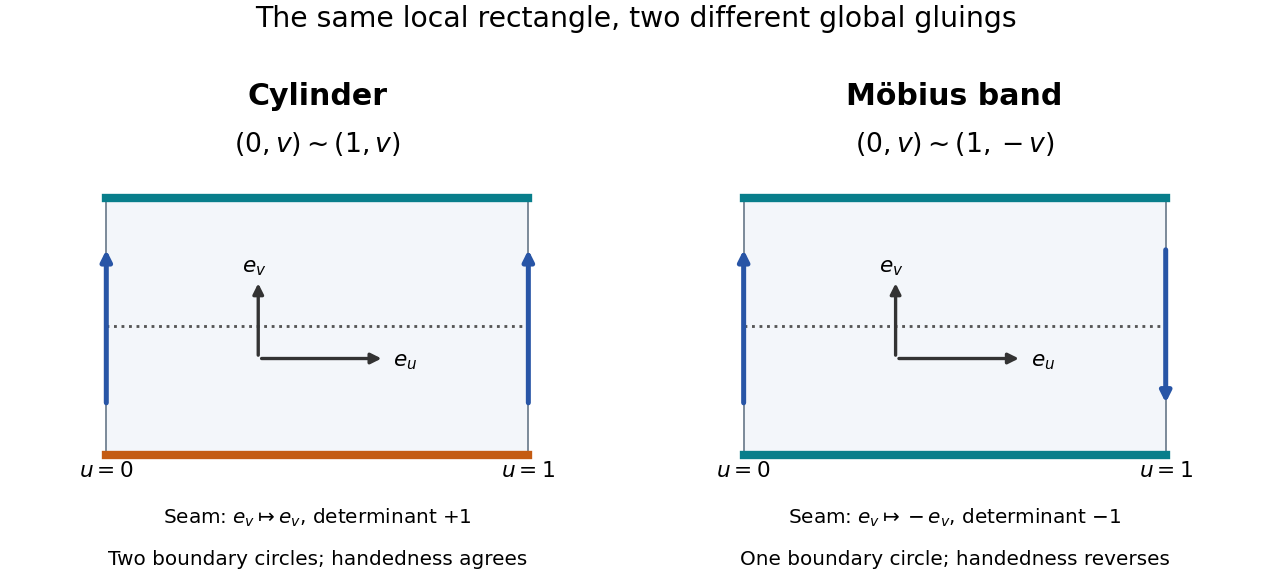


Both rectangles have coordinates . The untwisted band identifies with ; the Möbius band identifies with . Across a seam the corresponding local coordinate changes preserve or reverse , giving determinants and . This sign explains the handedness change; the drawing also tracks the two boundary circles of the untwisted band and the single boundary circle of the Möbius band.
For a smooth topological surface embedded in , choosing an orientation of a surface is equivalent to choosing a continuous unit normal. This picture is specific to surfaces in three-dimensional space: the general definition uses compatible local orientations, without requiring an embedding. Orientability is a topological invariant, so a homeomorphism cannot turn a Möbius band into a untwisted band. The sphere and torus are orientable surfaces; the Klein bottle is not. [ref]
The distinction matters when a sign has geometric meaning. A signed flux surface integral needs an orientation of a surface, and Stokes theorem relates that choice to the outward-normal-first boundary orientation. Ordinary unsigned surface area does not require orientability. Thus a Möbius band still has a perfectly meaningful area even though it has no continuous global unit normal.
A connected orientable manifold of positive dimension has two possible orientations: reversing every local choice gives the other one. If a manifold has several connected components, each component can be oriented independently when it is orientable. For topological surfaces, a useful obstruction criterion is the presence of a Möbius band: a surface is nonorientable exactly when it contains such a band. [ref]
https://pi.math.cornell.edu/~mec/Winter2009/Victor/part3.htm. Cornell Mathematical Explorers' Club, Orientable and Nonorientable Surfaces
Orientability of a regular fibre 2026-10-14
Choose an orientation of a vector space on . The quotient identification for a regular value gives a smoothly oriented normal bundle along . An oriented normal frame followed by a frame of defines the latter's orientation through the ambient orientation. Changing normal lifts adds only tangent components, so the determinant sign is unchanged. No orientation on all of is required.
Orientation of a simplex 2026-10-14
This simplicial notion is induced by an orientation of a vector space on the affine span of the simplex.
Orientation of a smooth manifold 2026-10-14
An orientation of a smooth manifold is a continuous choice of orientation of a vector space in every tangent space, equivalently an orientation of a vector bundle on its tangent bundle. It can be specified by an atlas with positive Jacobian determinants on all overlaps or by a nowhere-vanishing top-degree differential form. On a connected orientable manifold there are two choices, interchanged by reversing every tangent-space orientation.
// Target: differential-geometry.bigb
Orientation-preserving general linear group Created 2026-10-18 Updated 2026-10-25
The real invertible matrices with positive determinant form a subgroup of the general linear group. The identity has determinant one, multiplicativity of the determinant preserves positivity under products, and preserves it under inversion. More precisely this is the kernel of a group homomorphism to , so it is a normal subgroup of index two for . Its elements preserve an orientation of a vector space.
Oriented atlas 2026-10-14
An oriented atlas is a smooth atlas whose smooth transition maps have positive Jacobian determinants on every overlap. The coordinate bases then give compatible choices of orientation of a vector space on all tangent spaces. A nowhere-vanishing top-degree differential form gives such an atlas: restrict each chart until its coefficient has constant sign, reverse one coordinate if necessary to make that sign positive, and compare the positive coefficients on overlaps. Conversely, a partition of unity glues positive local coordinate top forms to a global volume form.
Past exam of the geometry of surfaces course of the University of Oxford 2023 2 e Solution 2026-10-25
The dihedral group here has order . Substituting into part (d) givesIn particular, requires genus seven. A geometric construction is to start with a round solid torus about the vertical axis, then drill thin radial tunnels through its tube in the horizontal midplane, equally spaced at azimuths , . The tunnels run from the central opening to the exterior; their directions are horizontal and radial. Round all their rims in the same way, preserving the dihedral symmetry, and let be the boundary of the resulting solid.
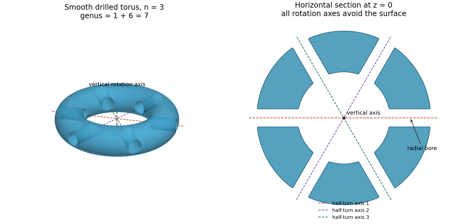
A genus-seven surface with a free dihedral action: six radial bores contain the horizontal rotation axes
. Details. 
Here is why the construction has exactly the required properties. Every nonidentity power of is a rotation in three dimensions fixing the vertical axis, which lies in the central opening and is disjoint from . Each element is a half-turn about a horizontal line at azimuth , modulo . The such lines meet the original solid torus in short radial segments. Each segment lies strictly inside one drilled tunnel, so these axes are also disjoint from . A nonidentity rotation in three dimensions fixes only its axis. Thus no nonidentity element fixes a point of , proving a free action of a group.
Rotation by permutes the tunnels, while preserves their arrangement and the original solid torus. Hence is preserved by the two generators and therefore by . The tunnels can be chosen sufficiently thin to be pairwise disjoint, and the rounding can be made group-invariant in small disjoint neighbourhoods of their rims. It neither changes the genus nor introduces an intersection with any axis.
Each tunnel removes two discs from the existing boundary and inserts the cylindrical wall of the bore. Its contribution to Euler characteristic is : the two removed discs contribute , and the inserted annulus and its boundary circles have zero Euler characteristic. The boundary remains connected and orientable, so each tunnel increases genus by one. Starting from a torus and drilling tunnels therefore gives . The construction also supplies a Riemann surface: use the complex structure associated with the induced oriented Riemannian metric. The ambient generators are isometries preserving the solid and ambient orientation of a vector space, so they preserve the induced boundary orientation and act by biholomorphisms. Part (d) then confirms that the quotient space has genus two. This is a free dihedral action on a drilled torus.
Past exam of the mathematical methods I course of the University of Oxford 2019 12 c Solution 2026-10-25
In a real orthonormal basis, a matrix is a proper rotation matrix exactly when and . The first condition preserves dot products, and the second preserves orientation of a vector space.
Put , , and , so the rows of the given matrix are . Their squared Euclidean norms and pairwise dot products areThus . For the sign of its determinant, use the circulant form:This proves that it is a rotation matrix. Its fixed axis is , because each row sums to one. The rotation trace formula gives ; the skew part selects a positive angle about the unit axis .
The original triangle has edge vectors and . Its area is half the Euclidean norm of their cross product:The rotated vertices are twice the three columns of :A rotation matrix preserves lengths and the angle between the two edge vectors, so it preserves their parallelogram area. More explicitly, for a proper rotation matrix, and , so the rotated edge cross product is again . Therefore
Past exam of the mathematical methods I course of the University of Oxford 2021 resit 9 ii Solution 2026-10-25
Label opposite , opposite , opposite and opposite . Since the tetrahedron is nondegenerate, its scalar triple product is nonzero. Put to handle either orientation of a vector space. Then the required outward vectors areEach cross product has magnitude twice the area of its triangular face. The signs are fixed geometrically: , so points away from the opposite vertex; the same test with and handles and . For the remaining face, the displacement toward its opposite vertex is , and , again outward.
Expand the first cross product:ThereforeThis is closure of outward face area vectors, with every face area multiplied by the same factor two. Omitting would orient all four faces inward when .
Past exam of the mathematics course of the University of Cambridge 2005 iii Paper 15 2 Solution Created 2026-10-03 Updated 2026-10-14
A -dimensional embedded submanifold has the subspace topology and, near each of its points, a manifold chart identifying it with a coordinate slice . These slice charts for an embedded submanifold give its smooth structure, and its inclusion is a smooth embedding.
A regular value of a smooth map is one for which is surjective at every . If the preimage is nonempty this forces .
The inverse function theorem used here says that if is smooth and is an invertible matrix, then its restriction to a suitable neighbourhood of is a diffeomorphism onto an open neighbourhood of , with smooth inverse.
To prove the regular level set theorem, fix and choose coordinates centred at . The coordinate representative has a rank- Jacobian matrix. After permuting domain coordinates, its first columns form an invertible matrix. DefineIts Jacobian matrix is block triangular with invertible diagonal blocks, so the inverse function theorem makes a local coordinate change. In these coordinates, is precisely the slice with first coordinates zero. Thus it is an embedded submanifold of dimension , withAn empty preimage is harmless; the local assertion is then vacuous.
Three equivalent formulations of orientability of a smooth manifold are: an oriented atlas whose transition Jacobian determinants are positive; a smoothly varying orientation of a vector space on each tangent space; and a nowhere-vanishing smooth top-degree differential form. An oriented atlas gives compatible oriented coordinate frames. A partition of unity glues their positive local top forms, and a nonzero top form declares a frame positive precisely when it evaluates positively on that frame. These constructions prove the equivalence.
For the orientability of a regular fibre, write . The derivative gives a short exact sequence of vector bundlesThis is the reason the normal bundle of a regular fibre is trivial. Choose any fixed positive basis of and an ambient orientation on . Declare a frame of positive whenis positive in , where . Changing a lift adds a tangent vector and leaves the determinant sign unchanged. Local smooth lifts exist because is surjective, so this rule varies smoothly and agrees on overlaps. It gives a global orientation on . Only an orientation of the single vector space was chosen; itself need not be orientable.
Past exam of the mathematics course of the University of Cambridge 2005 iii Paper 25 5 Solution Created 2026-10-03 Updated 2026-10-14
The smooth h-cobordism theorem states: if is a compact smooth h-cobordism, , and its connected boundary manifolds are simply connected, then there is a diffeomorphism restricting to the prescribed identification on . In particular and are diffeomorphic. Being an h-cobordism means that both inclusions are homotopy equivalences; their fundamental groups then also identify with that of .
The homotopy-equivalence condition is necessary for a trivial cobordism: each end of a cylinder is a deformation retract, by for the incoming end and for the outgoing end. Its relative homology with respect to either end is consequently zero. Compactness is also necessary for a product with a closed compact end. The dimensional bound and simple connectivity are not necessary for an individual cobordism to be a product. The cylinder is a simply connected trivial cobordism of dimension three; and, in the theorem's dimension range, is a six-dimensional trivial cobordism with fundamental group . These prove the two non-necessity assertions explicitly, while the inclusion argument proves necessity of the h-condition.
For the remaining claims, use a cobordism Morse function: its two regular boundary levels are zero and one, and all critical points are interior. An arbitrary function with unrelated boundary values would not have the relative handle-count property. The relative Morse chain complex for has one generator per critical point, in its Morse index. ThusA trivial cobordism has zero relative homology, hence zero relative Euler characteristic. Modulo two the displayed sum is the number of critical points. An odd number makes it odd, and therefore nonzero. This proves an odd-critical-point cobordism is not trivial.
With precisely two critical points of indices , a trivial cobordism requires the two-generator relative complex to be acyclic over . Equal indices leave a rank-two homology group; a gap of more than one leaves both generators with zero possible differential. Therefore is necessary. The remaining two-term complex isChoose a transverse gradient-like vector field. A nonzero differential requires the index- point to be above the index- point; otherwise no descending connecting trajectories exist. In a common regular level between them, the belt sphere has dimension , and the attaching sphere has dimension , where . Their dimensions add to , the level's dimension, so their transverse intersection consists of points. Each intersection is one descending trajectory from to , modulo time translation. Orient the attaching sphere and use an orientation of a vector space on the handle core to coorient the belt sphere; the resulting signed count is the cellular boundary coefficientThe two homology groups are the kernel and cokernel of multiplication by . They vanish precisely when is a unit of . Consequentlyare necessary. This proves the two-critical-point obstruction to a trivial cobordism; it makes an algebraic incidence statement and does not assume that an algebraic count of one automatically supplies geometric handle cancellation.
For an explicit nontrivial cobordism from to itself, attach two zero-framed two-handles to the outgoing end of along the standard Hopf link. Its two components are unknots with linking number one. This realizes two successive surgeries, as suggested by the hint. The outgoing boundary is again , and this can be checked geometrically: the Hopf-link exterior is , and each component's zero-framing longitude is the other's meridian. Filling along these two slopes glues two solid tori with meridians intersecting once, the standard genus-one Heegaard decomposition of . Thus zero surgery on the Hopf link does return the three-sphere, not just an unspecified homology sphere.
The trace has only the two added index-two handles. Its relative cellular complex has and all other groups zero, soIt cannot be a product cylinder. Equivalently this trace is with two disjoint open four-balls removed: the usual handle presentation of has one zero-handle, the two zero-framed Hopf-linked two-handles, and one four-handle. Removing the bottom and top balls exposes the two three-sphere ends. The relative-homology calculation alone already proves the requested cobordism is nontrivial.
Past exam of the mathematics course of the University of Cambridge 2010 iii Paper 15 3 a Solution Created 2026-10-03 Updated 2026-10-14
An oriented atlas is a smooth atlas whose smooth transition maps have positive Jacobian determinants at every point of their domains. Such an atlas supplies an orientation of a vector space on every tangent space, and these choices agree on overlaps.
Let be a nowhere-vanishing smooth top-degree differential form. In a coordinate chart writeThe coefficient is smooth and nowhere zero. Restrict the coordinate chart to connected neighborhoods; the intermediate value theorem makes the sign of constant on each. If is negative, replacing by changes the sign of the coordinate volume form. Thus for we can choose a covering of coordinate charts in each of which the coefficient is positive.
On an overlap of two such coordinate charts, the wedge product of differential forms transforms byConsequently . Both coefficients are positive, so the Jacobian determinant is positive, as is that of the inverse transition. A nowhere-vanishing top form therefore determines an oriented atlas. The zero-dimensional case has only zero-dimensional transitions, whose determinant is one, and is automatically orientable. Connectedness of is not needed for the positive-dimensional construction; only the local sign choice matters.
Rotation matrix Created 2026-09-24 Updated 2026-10-14
A rotation matrix turns vectors while preserving their shape relationships. For column coordinate vectors in an orthonormal basis, its defining conditions arewhere is the transpose and the identity matrix. In the usual Cartesian basis of the plane, an active counterclockwise planar rotation through an angle usesHere the vector moves and the basis stays fixed: . Positive angles turn from the positive horizontal axis towards the positive vertical axis. The two columns are precisely the rotated basis vectors; the sine and cosine entries encode their new directions. Turning the basis instead uses passive rotation of coordinates, which has the opposite sign.
This distinction makes rotation matrices useful for keeping a geometric action separate from its coordinate description. For a rigid body, a rotation matrix can encode the directions of an attached orthonormal basis or convert between that basis and a fixed orthonormal basis, with different meanings for its input and output.[ref]
Modern Robotics: Mechanics, Planning, and Control by Kevin M. Lynch and Frank C. Park. Modern Robotics, §3.2.1.2, preprint p. 69: three uses of a rotation matrix
The orthogonal matrix condition preserves every dot product:Consequently Euclidean norms and angles between nonzero vectors are preserved, as is the Euclidean norm of the difference between any two endpoints. The additional determinant condition preserves orientation of a vector space and oriented volume: for any square matrix whose columns are the input vectors, . An orthogonal matrix of determinant , such as a reflection matrix, preserves dot products but reverses orientation of a vector space. The matrix inverse is especially simple: .[ref]
Modern Robotics: Mechanics, Planning, and Control by Kevin M. Lynch and Frank C. Park. Modern Robotics, §3.2.1, definition 3.1 and propositions 3.3–3.6, preprint pp. 67–69
Signed curvature 2026-10-14
Fix the standard orientation of a vector space on the plane. For an oriented regular curve in that plane, let be its unit tangent vector and let be its left unit normal, obtained by an anticlockwise rotation through . Its signed curvature , also commonly written , is defined byHere increases with the chosen traversal and is the determinant. Positive signed curvature means turning left; negative signed curvature means turning right. The left unit normal exists even when ; when it points opposite to the principal normal vector. See Ghomi's university lecture notes, section 1.10.
For an arbitrary regular parametric curve traversed with increasing , the signed curvature isFor the anticlockwise circle , the numerator is and the denominator is , so . For the clockwise traversal , the numerator is , so , while unsigned curvature is in both cases. On this circle points inward for anticlockwise traversal and outward for clockwise traversal. For any simple closed regular curve traversed anticlockwise, is the inward unit normal, but signed curvature can still be negative along nonconvex portions.
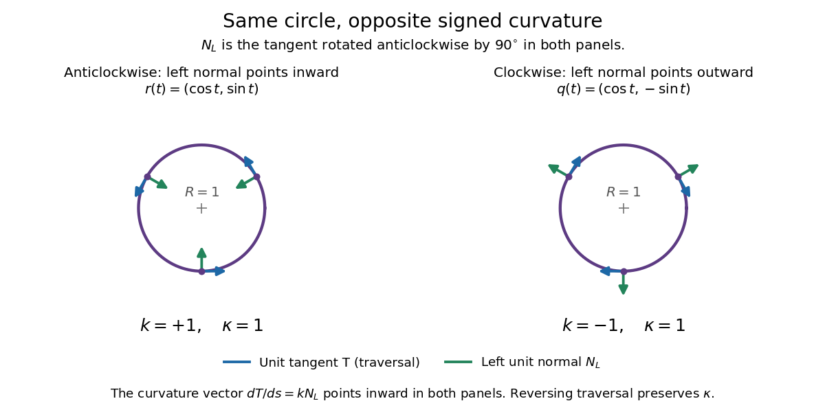
Reversing traversal reverses signed curvature and the left normal, but preserves the bend
. Details. 
To see why the formula uses the cube of the speed, write and . The term parallel to contributes zero to the determinant, giving . Under a reparametrization with , the numerator gains a factor and the denominator gains . Thus orientation-preserving reparametrization preserves signed curvature, while reversing traversal changes its sign at corresponding points. Unsigned curvature is preserved in either case.
Locally write the unit tangent vector as . Differentiating with respect to arc length gives : signed curvature records the direction as well as the amount of turning. Its integral therefore measures net turning, as in the turning tangent theorem; the integral of is total curvature and counts both left and right turns positively.