Past exam of the classical mechanics course of the University of Oxford / 2023 (B7.1, A14684W1)

Solutions to all three questions of the University of Oxford Part B classical mechanics examination, sat on 16 June 2023. Source: original released PDF, bundle pages 260–263; paper pages 1–4.

Each simple pendulum moves in the vertical plane containing the pivots. Ignoring contact between the ideal rods and point masses, each rod can turn through a full circle. Thus the configuration space is the torusChoose generalized coordinates ${\theta }_1,{\theta }_2$, measured from the downward vertical, positive towards the right and understood modulo $2\pi$. These angles are local coordinates on the torus, rather than a single globally one-to-one real coordinate chart. With upward Cartesian coordinate $y$, the bob positions areTheir velocities satisfy $|{\dot{\mathbf{r}}}_j{|}^2=l^2{\dot{\theta }}_j^2$, so kinetic energy from Cartesian position vectors givesThe spring length is the Euclidean distanceTaking gravitational potential energy zero at pivot height gives $V_g=-mgl(\cos {\theta }_1+\cos {\theta }_2)$. The spring potential energy is $V_s=k(d-r{)}^2/2$, since $r$ is its natural length. Consequently the Lagrangian isIn the paper's notation $t({\theta }_1,{\theta }_2)=V_s$; this function is distinct from the time variable. This is the exact Lagrangian of two spring-coupled pendulums.

One alternative Lagrangian isIt corresponds to setting gravitational potential energy zero at the downward position. The constant disappears from every Euler-Lagrange equation. More generally, total-time-derivative invariance of a Lagrangian allows $\tilde{L}=L+dF({\theta }_1,{\theta }_2,t)/dt$ for any smooth $F$.

Set $l=m=g=1$. At $({\theta }_1,{\theta }_2)=(0,0)$ the spring has $d=r$, so its potential energy has zero gradient: ${\partial }_j{V}_s=k(d-r){\partial }_{j}d=0$. The gravitational potential energy has ${\partial }_j{V}_g=\sin {\theta }_j=0$ there. Zero velocities therefore satisfy the Euler-Lagrange equations, proving this is an equilibrium.

For fixed $r>0$, let $\epsilon =\max (|{\theta }_1|,|{\theta }_2|)$ and $\delta ={\theta }_2-{\theta }_1$. The Taylor series giveThus, near the downward equilibrium, the horizontal separation is positive andIn particular, $V_s=k{\delta }^2/2+O({\epsilon }^4)$ and $V_g=-2+({\theta }_1^2+{\theta }_2^2)/2+O({\epsilon }^4)$. Dropping the additive constant and terms beyond quadratic order gives the harmonic approximationFor physical spring constant $k\ge 0$, the quadratic potential energy is a positive-definite quadratic form. The downward position is therefore a stable equilibrium in Lagrangian mechanics, and its nearby motion admits small oscillations.

The Euler-Lagrange equations of the quadratic Lagrangian areThe mechanical mass matrix is the identity. A normal mode $\mathbf{\theta }=\mathbf{a}\cos (\omega t+\varphi )$ therefore satisfies the eigenvalue problem $\mathsf{K}\mathbf{a}={\omega }^2\mathbf{a}$. Direct multiplication givesThese are normal modes of two spring-coupled equal pendulums. The corresponding normal mode coordinates $u={\theta }_1+{\theta }_2$ and $v={\theta }_1-{\theta }_2$ obey $\ddot{u}+u=0$ and $\ddot{v}+(1+2k)v=0$.

For the in-phase normal mode, the bobs undergo identical displacements, leaving their separation exactly $r$. The spring stays at its natural length and exerts no force, so this angular frequency is independent of $k$. The value $1$ is the individual simple pendulum angular frequency $\sqrt{g/l}$ in the chosen units.

Write $w=\sqrt{1+2k}$. The initial conditions on the normal mode coordinates are $u(0)=v(0)=0$ and $\dot{u}(0)=\dot{v}(0)=k$. Solving the two harmonic oscillator equations and recovering the original angles gives the exact solution within the harmonic approximation:Their angular velocities are ${\dot{\theta }}_1=k(\cos t+\cos wt)/2$ and ${\dot{\theta }}_2=k(\cos t-\cos wt)/2$, which verify all four initial conditions.

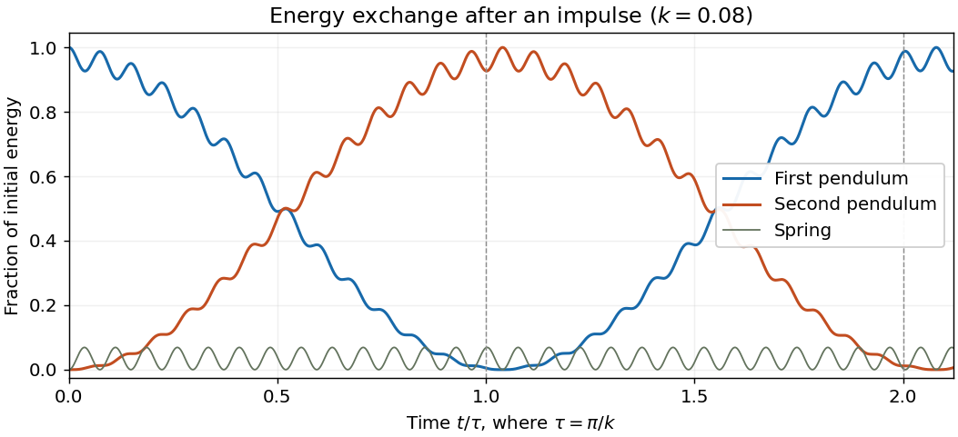
To expose the beat, define $\Delta =w-1$ and $\Omega =(w+1)/2$. Replacing $1/w$ by $1$ changes each angle by $O(k^2)$ uniformly in time. The sum-to-product identities then giveThe displayed angular velocities are exact in the linear system. The absolute and signed beat envelopes have leading amplitudes $k|\cos (\Delta t/2)|$ and $k|\sin (\Delta t/2)|$. Because $\Delta =k+O(k^2)$, at $\tau =\pi /k$ we have $\Delta \tau /2=\pi /2+O(k)$ and $\Omega \tau =\tau +\pi /2+O(k)$. HenceThe first simple pendulum has negligible oscillation amplitude. Its kinetic energy is $T_1(\tau )=O(k^4)$, while the second has $T_2(\tau )=k^2{\cos }^2\tau /2+O(k^3)$. Thus, to the retained order, all instantaneous kinetic energy belongs to the second simple pendulum. The fast phase can make that kinetic energy small: the whole initial energy $k^2/2$ is transferred as the second simple pendulum's combined kinetic energy and gravitational potential energy, sinceThis is energy transfer after an impulse in two weakly coupled oscillators. It does not require $\cos \tau =1$.

At $2\tau$, $\Delta (2\tau )/2=\pi +O(k)$, so the beat has returned the oscillation to the first simple pendulum:The energy localization returns, although the fast oscillation phase need not equal its initial phase. The exact first minimum of the leading beat envelope is at $\pi /\Delta$, whose leading value is $\pi /k$. Keeping the slow phase $\Delta t$ is essential: expanding $\sin (wt)$ at fixed $t$ and then using $t=O(1/k)$ would lose the energy exchange. Although angles are retained only to order $k$, their leading energies are of order $k^2$.

Take the origin at the centre of mass, so ${\int }_B\rho \mathbf{r}{d}^{3}r=0$, and write $r_i=\mathbf{r}\cdot {\mathbf{e}}_i$ in the specified orthonormal basis. The inertia tensor isHere ${\delta }_{ij}$ is the Kronecker delta. For a rigid body with angular velocity $\mathbf{\omega }$, this tensor gives $\mathbf{L}=\mathbf{I}\mathbf{\omega }$ and rotational kinetic energy $T=\mathbf{\omega }\cdot \mathbf{I}\mathbf{\omega }/2$.

The inertia tensor is a real symmetric matrix, so it admits an orthonormal basis of eigenvectors. The lines in these eigenvector directions through the centre of mass are its principal axes; the corresponding eigenvalues $I_1,I_2,I_3$ are its principal moments of inertia:If an eigenvalue repeats, the corresponding principal axes need not be unique.

Put $\mathbf{r}=(x,y,z)$ with ${\mathbf{e}}_3$ along $z$, and interpret the symmetry as axisymmetry of the whole mass density. A half-turn about ${\mathbf{e}}_3$ sends $(x,y,z)$ to $(-x,-y,z)$ and leaves the integration domain and mass density invariant. Therefore $\int \rho xz{d}^{3}r=\int \rho yz{d}^{3}r=0$. A quarter-turn sends $(x,y,z)$ to $(-y,x,z)$; it givesAll off-diagonal entries of the inertia tensor consequently vanish. Writing $s^2=x^2+y^2$, the principal moments of inertia satisfyThus every orthonormal basis with third vector along the symmetry axis is a principal body frame. This is axisymmetry of the inertia tensor. In general there is no requirement that $I_3=I_1$.

For a vector $\mathbf{A}={\sum }_i{A}_i{\mathbf{e}}_i$ in the principal body frame, the derivative of a body-fixed basis vector is $(d{\mathbf{e}}_i/dt{)}_{\hat{S}}=\mathbf{\omega }\times {\mathbf{e}}_i$. Differentiating the expansion gives the rotating-frame derivative formula, also called the Coriolis formula:Apply this to angular momentum $\mathbf{L}={\sum }_i{I}_i{\omega }_i{\mathbf{e}}_i$. The principal moments of inertia are constant in the principal body frame, so external torque balance becomesResolving the cross product gives Euler's equations:All components and dotted components in this display refer to the principal body frame.

For the symmetric top, set $I_1=I_2=J$. The third of Euler's equations reduces to $I_3{\dot{\omega }}_3={\tau }_3=0$. Thus the axial angular velocity component is a conserved quantity:The transverse angular velocity components are generally variable. A torque constant in the principal body frame generally rotates in the inertial frame; constancy in the two frames is different.

Let $J=I_1=I_2$, ${\omega }_3=c$ andHere $c$ and $\nu$ are constant. The first two of Euler's equations give ${\dot{\omega }}_1=-\nu {\omega }_2+{\tau }_0/J$ and ${\dot{\omega }}_2=\nu {\omega }_1+{\tau }_0/J$. Combining them producesMultiplication by the integrating factor $e^{-i\nu t}$ gives, for $\nu \ne 0$,For completeness, $\nu =0$ instead gives $z(t)=z(0)+{\tau }_0(1+i)t/J$. These formulas describe a symmetric top under constant transverse body torque.

The stated initial conditions require $b\ne 0$ and $I_3\ne J$. They give $c=b/(I_3-J)$, $\nu =b/J$ and $z(0)=i{\tau }_0/b$. Substitution and simplification yieldTaking the real part and imaginary part, the angular velocity in the principal body frame isIts value at $t=0$ is the required initial condition; differentiating the first two components verifies both forced Euler's equations.

Now take zero torque and $\mathbf{\omega }(0)=(1,0,1)$. The axial angular velocity is ${\omega }_3=1$ and the complex transverse component obeys $\dot{z}=i\nu z$ with $z(0)=1$ and $\nu =(I_3-I_1)/I_1$. Hence the angular momentum components in the principal body frame areThe transverse projection therefore traces a circle with signed angular frequency $\nu$. Its magnitude is constant, $L=\sqrt{I_1^2+I_3^2}$.

In the inertial frame, zero torque means that $\mathbf{L}$ is fixed. Usingand the derivative of a body-fixed basis vector, the symmetry axis satisfiesThus there is uniform torque-free precession of a symmetric top about the fixed angular momentum, at a constant cone angle $\beta$ and space angular frequencyThe cone angle stays constant, with no nutation. The body-frame and space-frame frequencies of free symmetric-top precession differ: $\nu$ describes rotating components, whereas ${\Omega }_{\mathrm{space}}$ describes the symmetry axis in space. The formulas also cover $I_3=I_1$, where the angular momentum components in the principal body frame are constant.

Define the canonical momenta byTo obtain an ordinary unconstrained Hamiltonian, assume a regular Lagrangian: the velocity Hessian matrix $({\partial }^{2}L/\partial {\dot{q}}_i\partial {\dot{q}}_j)$ is invertible. The inverse function theorem then lets us solve locally for $\dot{\mathbf{q}}=\mathbf{v}(\mathbf{q},\mathbf{p},t)$. The phase space is the cotangent bundle $T^{\ast }\mathcal{Q}$, with local canonical coordinates $(\mathbf{q},\mathbf{p})$ and dimension $2n$. The Legendre transform in mechanics definesThe velocities in this formula have been eliminated in favour of phase space variables. A hyperregular Lagrangian makes this construction global; regularity alone guarantees it locally. Hamilton's equations are

In canonical coordinates on phase space, the Poisson bracket isIt treats $t$ as a parameter. Along a solution of Hamilton's equations, the chain rule givesTherefore the Hamiltonian conservation law isThe total derivative follows the trajectory; the explicit partial derivative holds $(\mathbf{q},\mathbf{p})$ fixed.

The Poisson bracket is antisymmetric, so $\{H,H\}=0$. The Hamiltonian energy balance consequently givesFor a regular Lagrangian the Legendre transform in mechanics gives $H_t=-L_t$, evaluated at the corresponding velocity. In particular, a Lagrangian with no explicit time dependence has time-translation symmetry. Noether theorem associates this continuous symmetry of the action with the conserved quantity ${\sum }_i{\dot{q}}_i\partial L/\partial {\dot{q}}_i-L=H$. For an ordinary natural mechanical Lagrangian $L=T-V$, with $T$ quadratic in the velocities, this quantity is the total energy $T+V$.

Set $D={\partial }_t+\{\cdot ,H\}$. The hypotheses mean $Df=Dg=0$ as identities on phase space. By the Jacobi identity for the Poisson bracket,Also, the product rule applied to the defining coordinate formula givesAdding these identities provesConsequentlyThis proves the Poisson bracket of time-dependent conserved quantities theorem, including explicit time dependence of $f$ and $g$.

Since $H$ is a conserved quantity, the Hamiltonian energy balance gives $H_t=0$. Since $f$ is a conserved quantity, $f_t+\{f,H\}=0$. Take an explicit partial derivative with respect to time, holding the phase space coordinates fixed:The last Poisson bracket vanishes because $H_t=0$. ThusThis is the time derivative of a conserved quantity for an autonomous Hamiltonian. The conservation hypotheses are understood to hold for every trajectory, as identities on phase space.

The canonical momentum of the harmonic oscillator is $p=\partial L_0/\partial \dot{q}=m\dot{q}$. Substituting $\dot{q}=p/m$ into the Legendre transform in mechanics gives

Work on $I>0$, with a local choice of the periodic angle $\theta$. The inverse formulas areIn particular, ${\theta }_q=p/(2I)$, ${\theta }_p=-q/(2I)$, $I_q=\alpha q$ and $I_p=p/\alpha$. Their Poisson bracket isThe other fundamental Poisson brackets vanish by antisymmetry. Thus this is a canonical transformation for every $\alpha >0$, on local charts away from the origin. At $I=0$ the angle is undefined.

In the new coordinates the harmonic oscillator Hamiltonian isFor $I$ to be a conserved quantity throughout phase space, Hamilton's equations require $\dot{I}=-{\partial }_{\theta }{H}_0=0$ identically. The two coefficients must coincide. For the usual $m>0$ and $\omega >0$, positivity of $\alpha$ selectsThese are harmonic oscillator action-angle variables; the action variable is $I=H_0/\omega$.

A type-two generating function for a canonical transformation uses the mixed variables $(q,P)$ and definesFor a local invertible canonical transformation, require $F_{2,qP}\ne 0$ so that $p=F_{2,q}(q,P)$ can be solved for $P$. The differential identity $d{F}_2=pdq+QdP$ gives $d(F_2-PQ)=pdq-PdQ$, expressing preservation of the canonical symplectic form.

On the interior of the principal inverse-cosine branch, $0<q<\pi$, the given canonical transformation hasIntegrating $Q={\partial }_P{F}_2$ suggests $F_2=\cos q\sin P+C(q)$. Its other derivative is ${\partial }_q{F}_2=-\sin q\sin P+C^{\prime }(q)$; comparison with $p$ requires $C^{\prime }(q)=0$. Hence a suitable type-two generating function for a canonical transformation isBoth derivative equations reproduce the specified transformation exactly. Its mixed derivative is $F_{2,qP}=-\sin q\cos P$, so it defines a local canonical transformation where $0<q<\pi$ and $\cos P\ne 0$, equivalently where $|Q/\cos P|<1$. At $q=0,\pi$ or $\cos P=0$, the stated formulas fail to give a regular coordinate chart. These restrictions explain the square-root branch and the local meaning of canonicity. This is a trigonometric type-two canonical transformation.

For a time-dependent type-two generating function for a canonical transformation, the differential identitygives $K=H+{\partial }_t{F}_2$, with the partial derivative taken at fixed $(q,P)$. Here $F_2=\cos q\sin P$ has no explicit time dependence, so the Hamiltonian correction isAs always, adding a function of time alone to the new Hamiltonian leaves Hamilton's equations unchanged. Choosing a time-independent type-two generating function for a canonical transformation fixes that irrelevant freedom and gives the displayed $\Lambda =0$.