Past exam of the mathematical and Computational Biology course of the University of Cambridge / 2025

It tests whether the input string is a palindrome: reversing the characters leaves the string unchanged. Comparisons are case-sensitive and include spaces and punctuation. For example, mystery1("level") returns True, whereas mystery1("lever") returns False.

It performs a trial division test for a prime number. An integer below $2$ is rejected; otherwise the function searches for a divisor from $2$ through $\lfloor \sqrt{n}\rfloor$. A composite number has a prime factor no larger than its square root, so finding no such divisor proves primality. For example, mystery2(97) returns True, while mystery2(91) returns False, since $91=7\cdot 13$.

This describes the intended mathematical test. For extremely large integers, the floating-point computation n**0.5 can round or overflow; an implementation intended for arbitrary-size integers should use an exact integer square root.

It filters the first list by membership in the second list, retaining the order and all repetitions of qualifying entries in the first list. For example, mystery3([3, 1, 3, 2], [3, 4]) returns [3, 3]. Thus it is related to set intersection, but its result is a list and does not discard repeated elements.

With its default argument and a nonnegative integer input, it prints the decimal digits of $n$ in order, one per line. For example, mystery4(407) prints 4, then 0, then 7. Integer division removes the final digit, recursion handles the preceding digits, and the remainder gives the final digit. The function returns None.

There is a subtlety for a nondefault base: the recursive call omits m, so it resets to $10$. For $m\ge 2$ and $n\ge m$, the actual output is the decimal digits of $\lfloor n/m\rfloor$, followed by the remainder $n\mathrm{mod}m$. For example, mystery4(13, 2) prints 6, then 1, rather than the binary digits of $13$. Passing m on to the recursive call would give a consistent base-$m$ positional notation. The interpretation as digits assumes $n\ge 0$ and $m\ge 2$; arbitrary integer arguments need not satisfy those conditions.

Using the probability density function of the Erlang distribution, the expected value isHere $u=\theta x$, and two applications of integration by parts give ${\int }_0^{\infty }{u}^2{e}^{-u}du=2{\int }_0^{\infty }u{e}^{-u}du=2$. The boundary terms vanish because exponential decay dominates these powers.

Put $S={\sum }_{i=1}^N{x}_i$. Since the observations are independent random variables, their joint probability density function is a product. Therefore the likelihood function and log-likelihood areThese expressions assume positive observed values, as occurs with probability one under this continuous Erlang distribution.

The score function and the observed Fisher information areSolving the score equation gives the maximum-likelihood estimateThe positive observed Fisher information means that the log-likelihood is strictly concave on $\theta >0$. Its unique stationary point is therefore the global maximum. Equivalently, the score function changes from positive to negative at this point. At the estimate, $j(\hat{\theta })=S^2/(2N)$.

Test the null hypothesis $H_0:{\theta }_m={\theta }_f=\theta$ against the alternative hypothesis that the two rate parameters differ. Under $H_0$, the pooled maximum-likelihood estimate is ${\hat{\theta }}_0=16/36.8\simeq 0.434783$. Under the alternative, the estimates are ${\hat{\theta }}_m=8/22\simeq 0.363636$ and ${\hat{\theta }}_f=8/14.8\simeq 0.540541$.

In the likelihood-ratio test statistic, the data-only terms cancel, and both fitted models have total $\hat{\theta }S=16$. Consequently,The alternative hypothesis adds one parameter, so Wilks theorem gives an approximate chi-squared distribution with one degree of freedom. Do not reject the common-rate model at the 5% level, since $T<3.841$. The corresponding approximate p-value is $0.43$. The fitted expected values are $5.5$ and $3.7$ days, but four observations per group supply little evidence that the underlying expected values differ; failure to reject does not establish equality. The chi-squared distribution calibration is asymptotic and should be treated cautiously for these small samples.

The vector of column sample means is $\bar{x}=(1,3,2)$. Subtract it from each observation. The centred data matrix, with cell types in the original order, isEach column now has sample mean zero.

Using divisor $n=4$, the covariance matrix isFor example, the first variance is $(1+1+1+9)/4=3$, and the first-second covariance is $(3-1-1+3)/4=1$. If “sample covariance matrix” means the unbiased convention, use divisor $n-1=3$ instead: $S=(4/3)\Sigma$. This multiplies every eigenvalue by $4/3$ and leaves all principal component loadings and explained-variance fractions unchanged.

The total variance is the trace $\mathrm{tr}\Sigma =10$. Retaining two original genes preserves the sum of their marginal variances; the largest choice includes the third gene and either of the first two, giving $4+3=7$. Thus the largest proportion is 70%. This refers to retaining measured coordinates themselves, rather than replacing them by linear combinations as in principal component analysis.

The eigenvector $(1,-1,0{)}^{\mathsf{T}}$ has eigenvalue $2$. On its orthogonal complement, write vectors as $(a,a,c{)}^{\mathsf{T}}$. The eigenvalue equation becomesHence the ordered eigenvalues of the covariance matrix are $4+2\sqrt{2}$, $2$, and $4-2\sqrt{2}$. The first two principal components explainof the total variance. The denominator is the sum of all eigenvalues, which equals the trace.

The second-largest eigenvalue is $2$, with eigenvector $(1,-1,0{)}^{\mathsf{T}}$. A unit principal component loading is thereforeIt is orthogonal to the first loading $u_1=(1,1,\sqrt{2}{)}^{\mathsf{T}}/2$. Either sign of a loading is equivalent, provided its principal component scores use the same sign convention.

The centred observation for D is $d=(3,1,2{)}^{\mathsf{T}}$. Taking inner products with the unit principal component loadings gives its principal component scores:Normalizing the loadings matters: a direction alone does not fix the scale of the coordinates.

After subtracting the same training sample mean, E has vector $e=(1,-1,0{)}^{\mathsf{T}}$ and principal component scores $(0,\sqrt{2})$. The difference from D lies entirely along the first principal component. Its Euclidean distance in the retained plane isThe new point must use the original centring and loadings; recomputing them with E included would change the question.

For observation $j$ of bird $i$ in year $t(i,j)$, a Gaussian linear mixed model with crossed random intercepts iswhere the $u_i$, $v_t$, and ${\epsilon }_{ij}$ are mutually independent random variables. Here $a_{ij}$ is age, ${\beta }_0$ is the population intercept at age zero, and ${\beta }_1$ is the change in conditional expected value per year of age. The $u_i$ capture persistent between-bird variation, the $v_t$ capture shared annual conditions, and the regression residuals capture remaining observation-level variation. Two observations from the same bird share covariance ${\tau }_b^2$; two from the same year share ${\tau }_y^2$, with both contributions present if both group labels agree. The model also assumes the random effects are independent of the age covariate.

Conditional predictions for observed birds and years add their fitted random intercepts to the fixed part of the Gaussian linear mixed model:These are predicted expected values, so they need not be integers. The first is likely more reliable: age three is within the displayed age range, whereas age seven requires extrapolation beyond ages one to six. A quantitative comparison would need the prediction intervals, including uncertainty in both fixed coefficients and random effects; the displayed coefficients alone do not supply them.

The deviance entries are $-2\ell$ for these fitted models. The completed values areThe likelihood-ratio test compares a model with one age coefficient against its restriction ${\beta }_1=0$. Its small p-value, approximately $0.000529$, supports a positive age association under the assumed Gaussian linear mixed model. Refitting with maximum likelihood estimation is essential here: restricted maximum likelihood values from models with different fixed-effect design matrices cannot be compared by this likelihood-ratio test.

Yes. The bootstrap confidence interval for the age coefficient, $(0.057060,0.193584)$, excludes zero and supports the same positive association. A well-implemented parametric bootstrap can give better finite-sample calibration than the asymptotic likelihood-ratio test, especially with only eleven year groups and estimated variance components. Its advantage depends on simulating the full fitted Gaussian linear mixed model and refitting correctly; resampling individual records as if they were independent would discard the grouping. A bootstrap confidence interval is also not literally the same procedure as a bootstrap-calibrated test.

The bird-level standard deviation is appreciable, with interval $(0.436,0.720)$ hatchlings, whereas the year-level estimate is much less precise, with interval $(0.0195,0.333)$. The residual standard deviation is approximately $0.381$–$0.493$. Boundary fits in 23 of the 1000 replicates indicate that at least one fitted variance component sometimes reaches zero; the convergence warning should also be investigated before trusting the reported intervals. Neither the asymptotic test nor a model-based bootstrap repairs incorrect response-distribution or mean-structure assumptions.

“After accounting for bird identity and year using random intercepts, hatching success increased by an estimated 0.123 hatchlings per additional year of age (95% bootstrap confidence interval 0.057–0.194).”

This describes an observational association under the fitted Gaussian linear mixed model, rather than a causal age effect. The diagnostic assessment below is needed before treating this inferential statement as reliable.

The regression diagnostics raise concerns about the mean and variance assumptions. The residual-versus-fitted smoother is curved rather than horizontal, and the scale-location plot suggests changing residual spread, contrary to homoscedasticity. Diagonal bands are expected when an integer-valued response is fitted by a continuous model, since each fixed response value gives $r=y-\hat{y}$. They are not, by themselves, proof of a failed mean model. The residual Q-Q plot is broadly linear but has tail departures and unusual observations, so exact normality is questionable.

The Cook's distance plot identifies observations worth checking for recording errors and influence on the age estimate. A rough $4/n\simeq 0.023$ screening threshold flags several points, but it is not an automatic deletion rule. Repeat the fit with and without influential observations as a sensitivity analysis and report material changes.

The bird random intercept Q-Q plot has a pronounced upper-tail departure; the year plot is closer to a line, although eleven groups give little power to assess normality. These plotted effects are estimated, shrunken conditional mode of Gaussian random effects, not independent observed draws from the latent normal distribution, so their appearance requires care.

The analysis is therefore provisional. Check a nonlinear age effect, the changing residual variance, dependence beyond the fitted random intercepts, and a response model appropriate for counts. If clutch size is known, a binomial distribution model for hatched eggs out of available eggs may be more meaningful. A bootstrap from the existing Gaussian model cannot validate the assumptions questioned by these plots. Distinguishing within-bird ageing from between-bird differences would also strengthen interpretation.

The Poisson generalized linear mixed model assumes conditionally Poisson distributed counts with a log link. The fitted variance components are both zero, so this fit lies on a boundary and reduces to ordinary Poisson regression. It estimatesThus the fitted annual increase is about 6.6%, with approximate 95% confidence interval for the rate ratio $(e^{0.001},e^{0.128})\simeq (1.001,1.137)$. The age evidence is much weaker than in the Gaussian fit: the quoted p-value is $0.047$. Zero estimated group variances do not prove that real bird and year differences are absent.

The Poisson distribution forces conditional variance to equal the conditional expected value. Here fitted means are around two to three hatchlings, whereas the Gaussian model estimated a residual variance of only $0.188$. This suggests checking underdispersion and the bounded nature of hatching counts, rather than assuming a Poisson response solves the diagnostic problems. Inspect simulated count residuals and predictive distributions; if the number of eggs is observed, fit a binomial mixed model and check that model's dispersion too.

The displayed Gaussian and Poisson Akaike information criterion values should not simply be ranked as if they used the same likelihood convention: one evaluates a continuous density and the other a probability mass. Compare properly specified count models on the same observed response scale, with compatible likelihoods and predictive checks. A boundary fit, doubtful dispersion assumptions, and possible nonlinear age effects all warrant further work before a strong biological conclusion.

The product rule givesIn particular, the second derivative is negative throughout the domain.

The function is strictly concave on $x>0$. Its derivative is positive for $0<x<1$, zero at $x=1$, and negative for $x>1$. Thus it rises from the limiting value $-1$ as $x\downarrow 0$, touches the horizontal axis at its unique maximum $(1,0)$, and then decreases to $-\infty$. It never crosses above the axis. The left endpoint is not included, and the slope tends to $+\infty$ there.

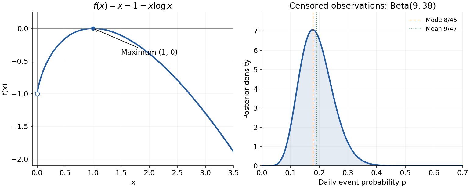
The left panel shows the required sketch; the right panel is used for question 6(e).

This is the Nicholson-Bailey model for a host-parasitoid interaction with discrete generations. The factor $r$ is the host multiplication factor in the absence of parasitism; $a$ measures effective attack or searching intensity per parasitoid; and $b$ is the number of next-generation parasitoids produced per attacked host, with any survival or unit conversion absorbed into it.

If the number of attacks on a host has a Poisson distribution with expected value $a{P}_t$, then the probability of no attack is $e^{-a{P}_t}$. Consequently $e^{-a{P}_t}$ is the surviving, unparasitized host fraction, and $1-e^{-a{P}_t}$ is the attacked fraction. The two update equations count host descendants from surviving hosts and parasitoid descendants from attacked hosts, respectively.

At an equilibrium, $H=rH{e}^{-aP}$ and $P=bH(1-e^{-aP})$. Taking $H=0$ forces $P=0$, giving extinction. If $H\ne 0$, the first equation gives $e^{-aP}=1/r$ and henceThese are the only isolated candidates obtained from the equations. There is an exceptional parameter case: at $r=1$, $P=0$ and every $H\ge 0$ is an equilibrium. Thus the assertion of exactly two equilibria needs $r\ne 1$, and only the positive candidate belongs to the biological state space when $r>1$.

Since $a,b>0$, the coexistence value $P_{\ast }=(\log r)/a$ is positive exactly when $r>1$. Under that condition, $H_{\ast }>0$ as well. Therefore the required condition isFor $0<r<1$, the formal nonzero candidate has negative parasitoid density and is not biologically admissible; $r=1$ gives only the host-only line of equilibria.

The Jacobian matrix of the update map isIts eigenvalues are $r$ and zero. The extinction equilibrium is locally asymptotically stable for $0<r<1$ and unstable for $r>1$, by linear stability analysis for a discrete dynamical system. In the latter case, even a small perturbation along $P=0$ grows as $H_t=r^t{H}_0$.

At $r=1$, an eigenvalue equals one, so the strict linear criterion does not decide stability. Directly, $0\le H_{t+1}\le H_t$ and $0\le P_{t+1}\le b{H}_t$. Starting sufficiently close to extinction therefore keeps both coordinates close for all time, proving Lyapunov stability in the nonnegative state space. It is not asymptotically stable, since every nearby $(H,0)$ is another equilibrium. This distinction makes the statement “stable when $r>1$ fails” precise.

Suppose $r>1$ and set $q=\log r/(r-1)$. Substitution of the positive equilibrium into the Jacobian matrix givesPart (b) showed $f(x)<0$ whenever $x\ne 1$. In particular,gives $\log r<r-1$, whereasgives $\det J_{\ast }>1$. The latter already violates the Jury stability criterion condition $1-\det J_{\ast }>0$. More directly, the product of the two eigenvalues is greater than one, so at least one has modulus greater than one. Therefore the positive equilibrium is unstable. This is the instability of the Nicholson-Bailey equilibrium; parasitoid feedback in this simple model does not stabilize coexistence.

For independent geometric random variables supported on $1,2,\dots$, put $S={\sum }_i{x}_i$. Multiplication of their probability mass functions gives the likelihood functionThere are $n$ terminal successes and $S-n$ preceding failures.

The beta distribution prior density is proportional to $p^{a-1}(1-p{)}^{b-1}$. By Bayes' theorem, its product with the likelihood function gives the posterior densityThis is again a beta distribution, namelyThus the beta family is a conjugate prior family for the geometric distribution. The update is an instance of beta-geometric conjugacy: counts of observed successes and failures are added to the two beta parameters.

Using the expected value of a beta distribution, the posterior mean isEquivalently, it is the weighted averageof the prior mean and the maximum-likelihood estimate $n/S$.

For fixed prior parameters, divide numerator and denominator by $n$:under independent sampling from a geometric distribution with true success probability $p_0>0$. The law of large numbers gives $S/n\to 1/p_0$. In a large finite sample the posterior mean is close to $n/S=1/\bar{x}$, the maximum-likelihood estimate. The fixed prior's influence vanishes, and the estimate is consistent.

The two colonies with no observed cheaters are right-censored after seven days. Each contributes $\mathrm{Pr}(X>7)=(1-p{)}^7$, not the probability of an event on day seven or eight. The four observed first events contribute four factors of $p$ and $(6-1)+(7-1)+(5-1)+(5-1)=19$ failures. Including the two censored exposures givesThe beta distribution prior therefore yieldsIts probability density function is proportional to $p^8(1-p{)}^{37}$ for $0<p<1$: it vanishes at both endpoints, is unimodal, and has its mode at $8/45\simeq 0.17778$. The right panel of the sketch in question 5(b) shows this moderately right-skewed density. The calculation assumes daily observations detect the first event and that stopping the experiment after seven days is independent censoring.

The trace has long, slowly changing stretches, indicating strong autocorrelation and poor exploration of the posterior distribution. The reported effective sample size of a Markov chain is only $36$, so the number of stored draws greatly exaggerates the information in the simulation. The potential scale reduction factor $\hat{R}=1.21$ is appreciably above one and does not support convergence between chains. The reported Monte Carlo standard error $0.04$ is also large relative to a posterior mean near $0.2$.

The exact beta distribution gives posterior mean $9/47\simeq 0.19149$ and standard deviationso the simulation's reported spread $0.11$ is another warning. Do not interpret its mean or interval estimates as reliable yet. Run multiple chains from dispersed starts, improve and tune the proposal or sampler, and use longer runs after adaptation. Recheck the traces, potential scale reduction factor, and effective sample size of a Markov chain. More iterations help only if the chain actually explores its target well; thinning alone does not fix poor mixing.

Direct independent sampling is preferable. The posterior distribution is the standard beta distribution $\mathrm{Beta}(9,38)$, for which exact posterior moments and standard random-number generators are available. For example, draw independent $U\sim \mathrm{Gamma}(9,1)$ and $V\sim \mathrm{Gamma}(38,1)$ with the same rate, and return $U/(U+V)$. This has the required beta distribution and avoids Markov chain Monte Carlo convergence problems. A correct, converged MCMC method could sample this target, but it is unnecessarily complicated here.

Write $n_k=|C_k|$ and suppose the cluster is nonempty. Expanding the Euclidean norm through its inner product givesSum over $x\in C_k$. The final term does not depend on $x$, so its sum is $n_k\Vert z-{\bar{x}}_k{\Vert }^2$, which proves the requested identity. This expansion is the starting point for the centroid sum-of-squares identity.

The centred observations sum to zero:By linearity of the inner product,This cancellation holds for every $z$.

Combining the first two parts gives the centroid sum-of-squares identityThe added term is nonnegative and, since $n_k>0$, vanishes exactly at $z={\bar{x}}_k$. Thus the unique minimizing centroid in this step of K-means clustering isAn empty cluster needs a separate algorithmic convention because its sample mean is undefined and its objective is identically zero.

Expanding the squared Euclidean distances givesFor distinct centroids, chooseA point assigned to $C_1$ has the displayed distance difference at most zero and therefore $w^{\mathsf{T}}x+b\ge 0$; assignment to $C_2$ gives the reverse inequality. The separating hyperplane is the perpendicular bisector of the line segment joining the two centroids. Points tied between them lie on that hyperplane. This is the nearest-centroid decision hyperplane.

The requested nonzero $w$ needs the additional assumption $z_1\ne z_2$. It does not follow from the stated algorithm alone. In one dimension, take $C_1=\{-1,1\}$ and $C_2=\{0\}$, whose centroids are both zero. A tie rule that retains previous assignments can leave this configuration after an iteration. The inequalities at $-1,1$ imply $b\ge |w|$, while the inequality at zero implies $b\le 0$, forcing $w=0$. Thus the unconditional nonzero-separator claim has this degenerate exception.

A cyclic rotation moves the first character to the end without changing the cyclic order of the remaining characters. Starting with the specified terminator-first row and repeatedly rotating left gives the following matrix; its row order is only a construction order, not a sorting order:Under lexicographic order, compare characters from left to right, using $\$<A<C<G$. The sorted cyclic rotation matrix is thereforeThe Burrows-Wheeler transform is the last column, read downwards, so the transformed string is

To invert the Burrows-Wheeler transform, begin with six empty rows. At every iteration prepend the supplied last-column characters in their fixed row order, then sort the resulting rows in lexicographic order. After $k$ iterations the rows contain the length-$k$ prefixes of the sorted cyclic rotations. For example, the first two iterations giveEach iteration works because sorting the preceding character together with the already reconstructed prefix restores the ordering of the next-longer prefixes. Six iterations give the completed matrixThe original linear string is the unique row ending in the terminator, henceAs a check, the reconstructed matrix's final column is precisely the supplied Burrows-Wheeler transform.

Use one-based row numbers, and write $F$ and $L$ for the first and last columns. The last-to-first mapping matches the $k$th occurrence of a character in $L$ to its $k$th occurrence in $F$: equal characters retain the ordering of their following suffixes. This lets us extend an interval of matching suffixes one character to the left without reconstructing the full strings.

Start with the last query character. Rows $5,6,7$ of $F$ contain C, so the interval of suffixes beginning with C is $[5,7]$. Within those rows, the A entries of $L$ are at rows $5$ and $7$. They are respectively the first and second A entries in all of $L$, and therefore map to rows $2$ and $3$ of $F$. These are exactly the suffixes beginning with AC. Reading their supplied positions gives matches starting at positions 11 and 3, or positions 3 and 11 in increasing genomic order.

The same calculation can be written as backward search. Let $C(c)$ count characters strictly smaller than $c$, and let $\mathrm{Occ}(c,r)$ count occurrences of $c$ in $L[1:r]$, with $\mathrm{Occ}(c,0)=0$. Prepending $c$ changes an inclusive interval $[l,r]$ toHere $C(\mathrm{A})=1$, $\mathrm{Occ}(\mathrm{A},4)=0$ and $\mathrm{Occ}(\mathrm{A},7)=2$, giving $[l^{\prime },r^{\prime }]=[2,3]$.

Build an FM-index: store the Burrows-Wheeler transform, cumulative character counts $C$, and a structure supporting fast rank queries for $\mathrm{Occ}(c,r)$. Then each step of backward search uses two rank queries instead of rescanning the last column. A wavelet tree or suitably checkpointed counts can supply these queries while keeping memory manageable. The counting cost is proportional to query length times the rank query cost, rather than repeatedly scanning the whole genome.^[ref]

To recover genomic positions, store a sampled suffix array and follow the last-to-first mapping to a sampled position, adding the number of steps taken. More samples trade storage for faster position recovery. Index character counts and sample positions, rather than storing the quadratic-size full cyclic rotation matrix.