An odd composite integer coprime to is a Fermat pseudoprime to base if . A Carmichael number is a composite integer satisfying this congruence for every integer coprime to . The Korselt criterion says that a composite is a Carmichael number exactly when it is squarefree and divides for every prime divisor of .
By the Korselt criterion, the prime factors are distinct. There cannot be just one prime factor, since a Carmichael number is composite. If there were exactly two, write with . Then , so , impossible because . Hence at least three distinct prime factors are necessary.
The prime factorization is , so it is composite and squarefree. Moreover , and all divide . The Korselt criterion therefore proves that 561 is a Carmichael number.
The complex Taylor theorem says that an analytic function has the expansionthroughout every disk centred at contained in . In particular it converges for , and uniformly on every smaller closed disk. The coefficients are uniquely its derivatives divided by factorials. The convergence radius can be larger if the function extends beyond the boundary of ; the theorem does not say that the given domain determines its exact radius.
An elementary geometric-series construction suffices, without assuming a general polynomial-approximation theorem. Rotate the square by a multiple of so that . Put with . Every point of the square then satisfies , whereasfor sufficiently large . Thus the whole square lies inside a disk centred at whose radius is less than . The other three ways can lie outside the square are handled by the indicated rotations, after which rotating back preserves polynomial form.
Now expandLet . The tail after degree is uniformly bounded by , tending to zero. Hence the displayed partial sums are the required uniform polynomial approximations. This is the Taylor series about a carefully chosen distant centre, rather than a potentially inadequate series about .
Suppose a connected subset contains distinct points . The distance function is -Lipschitz, and its image on is connected and contains and . It therefore contains the whole interval between those values. A Lipschitz map cannot increase Hausdorff dimension: taking images of arbitrarily fine covers multiplies their diameter powers by at most a fixed constant. Since a nondegenerate interval has Hausdorff dimension one, , contradicting . Thus every connected subset is a singleton, so is totally disconnected.
A Möbius transformation pairs two disks when it maps their boundary circles to one another and takes the exterior of the first disk onto the interior of the second. Two pairs of disks with disjoint interiors give the ping-pong lemma construction of a free two-generator group. Tangencies are allowed in the convention suggested by the question; this is often called a Tangent-disk Schottky group, rather than a strictly separated Schottky group.
Here is a concrete configuration that also makes the dimension argument precise. Take and . The first pairs the half-plane disks and , which are disks on the sphere tangent at infinity. The second pairs and , tangent at zero; their interiors are also disjoint from the half-plane disks. These pairings give a free discrete Kleinian group by ping-pong lemma, with a nonempty open fundamental region.
Set . Conjugating the subgroup generated by by gives matricesThe product of the second matrix with the first is . These are the standard parabolic generators of the principal level-two modular group, whose ideal-quadrilateral fundamental region tiles the upper half-plane and whose Kleinian limit set is the entire extended real line. Consequently the original group's Kleinian limit set contains the circle , as well as its image under , the distinct tangent circle .
It follows that the limit set has Hausdorff dimension at least one and is not homeomorphic to a circle. Indeed a proper subset of a circle cannot itself be a circle: after deleting a missing point it lies in a line, which cannot contain an embedded circle. A space containing two distinct complete circles thus cannot be homeomorphic to a single circle. This explains why dimension at least one does not force circle topology. The tangent-circle terminology is consistent with the primary discussion of T-Schottky configurations in arxiv.org/pdf/math/0701572 .
Reliable transmission at rate means that there is a sequence of binary block codes of lengths , message counts with , and decoding error probabilities tending to zero. The Shannon second coding theorem identifies the supremum of reliable rates with the channel capacity.
For a binary symmetric channel, the conditional entropy of the output given any input bit is . The output entropy is at most one bit and attains one for uniform input, so the maximum mutual information isAll rates strictly below are achievable, and rates above are not reliable; this states the supremum without claiming achievability of every boundary rate under every convention.
For very small , the capacity is close to one, with . At , the output is independent of the input and capacity is zero. For , flipping every received bit converts the channel to crossover probability ; its capacity is unchanged because . At the deterministic bit flip is perfectly reversible.
The first two commands create vectors of observed successes and corresponding numbers of trials. The next two create the class labels and convert them into an R factor, so the labels are treated categorically. The final command fits a grouped-binomial logistic regression, using the proportions as responses and trial totals as binomial weights, and prints its summary. The model is , with class a as reference.
The intercept estimates the log odds in class a. Its value corresponds to probability . The class-b coefficient is the estimated increase in log odds, about , so the fitted probability in class b is and the estimated odds ratio is . The printed standard errors measure uncertainty in these estimated coefficients. The z values are estimate divided by standard error: the intercept tests whether the class-a probability is , while the class-b z value tests equal class probabilities. The two-sided normal-reference P-value for the latter is about , so it is just above a conventional threshold; this is a borderline result rather than strong evidence of a class effect.
The residual deviance compares the fitted two-parameter model with the four-probability saturated model. Its value on residual degrees of freedom is small relative to a reference, with approximate tail probability . There is no evidence of lack of fit by that check. Four Fisher scoring iterations were needed for numerical fitting. These interpretations presume independent binomial counts and the usual large-sample approximations; weights here encode trial counts, not extra independent observations.
Set . The exact Hebbian learning rule givesThus the norm never decreases, and increases whenever the output is nonzero. Because learning is slow relative to input fluctuations, its averaged equation is , where is the input second-moment matrix. It is a covariance matrix only if the inputs have zero mean. Diagonalizing the positive semidefinite matrix gives components . Hence weights grow without bound whenever the initial vector has a component in an excited positive-eigenvalue direction. A vector entirely in , or identically zero input, is an important stationary exception.
For the modified Hebbian learning rule,It increases below and decreases above , without crossing that equilibrium. More precisely, for a nonzero initial norm,Under persistent excitation, meaning the integral tends to infinity, this givesWithout persistent excitation the limiting norm need not reach this value; zero weights remain zero. The quartic norm stabilization of Hebbian learning bounds the norm and supplies negative feedback at large amplitudes.
Averaging the fast fluctuations in givesThus a nonzero steady vector satisfiesIts direction is an eigenvector of the input second-moment matrix, and its magnitude is the square root of that eigenvalue. The zero vector is also a steady state and satisfies the displayed relation with . This is an averaged steady state; the microscopic fluctuating update need not vanish at each instant.
Unmodified Hebbian learning reinforces correlated input and output but has no mechanism limiting synaptic strength. The second rule adds activity-dependent negative feedback and stabilizes the norm at an input-scale-independent value, provided the input keeps exciting the output. The third has a cubic weight penalty independent of the instantaneous output; its equilibrium norm instead depends on the strength of the input second moment.
For the third averaged rule, an equilibrium along eigenvector has radial linearized eigenvalue and transverse eigenvalues . Thus a positive simple largest eigenvalue gives stable equilibria in its two opposite directions, whereas lower eigen-directions are unstable to larger components. With generic initial weights, it learns the dominant correlation direction, linking the rule to principal component analysis. These are idealized normalization and feature-extraction mechanisms, not claims that biological synapses implement these exact equations.
The fixed points are and . The Jacobian matrix isAt the origin its eigenvalues are , so it is a saddle with stable direction the y-axis. At either other fixed point, the characteristic polynomial is , giving eigenvalues . Thus both are stable foci. The nullclines are , and . In the right half-plane grows below and decreases above it; in the left half-plane these horizontal arrows reverse. Vertically, increases below and decreases above it.
A global argument determines the requested omega-limit sets, rather than guessing from the local phase portrait. For , use the quadratic-logarithmic Lyapunov function for a feedback systemIts sublevel sets are compact and bounded away from , so trajectories starting in either half-plane exist for all positive time and stay in such a set. Since decreases, it tends to a limit, and is constant on the omega-limit set. Every point of that set therefore has . Invariance then requires , so only the corresponding focus can occur. Also preserves its sign.
ConsequentlyOn , the exact solution is . The phase portrait below shows this stable axis, the nullclines and the spiral attraction in each half-plane.
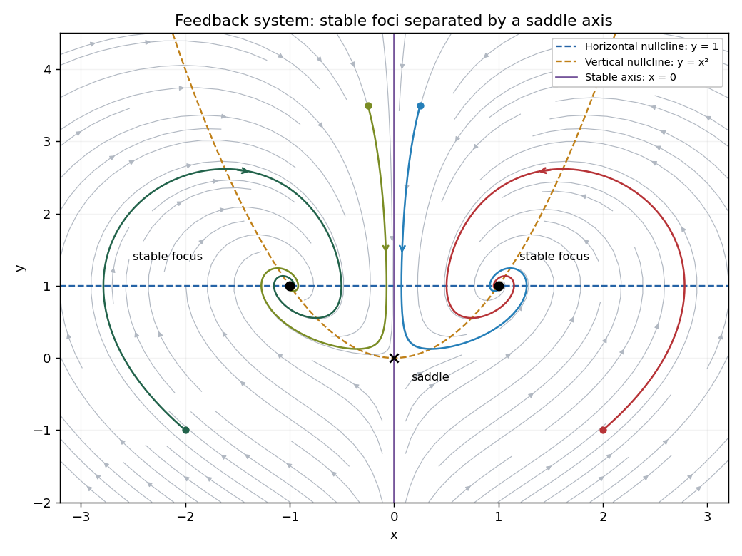
Phase portrait with a saddle at the origin and stable foci at plus or minus one, one
. Details. 
At zero an ordinary point requires to be analytic. A regular singular point requires and to extend analytically to zero, with at least one of failing to be analytic if “singular” excludes ordinary points.
Put and . Differentiation gives and , so the transformed equation isThe point at infinity is ordinary precisely when both transformed coefficients are analytic at . Solving these conditions for the original coefficients giveswith analytic near zero; the sign can be absorbed into the arbitrary analytic .
If the only singular point on the sphere is the regular singularity at zero, then and are entire. The condition at infinity makes the first tend to and the second to . By Liouville theorem they are respectively the constants and . Thus the unique equation iswith general solution . Zero is genuinely regular singular and infinity is ordinary. If “no other singular points” were restricted to finite points only, the general coefficients would instead be and with entire ; the preceding question about infinity indicates the spherical interpretation.
A one-dimensional canonical transformation is a locally invertible change of phase-space variables preserving the symplectic two-form: . Equivalently it preserves Hamilton equations for the transformed Hamiltonian. Expanding the two-form yieldssoConversely this Jacobian condition makes the transformation locally invertible and symplectic in two dimensions.
The Poisson bracket is . For it to be identically one on an open region, the exponent must vanish and the coefficient must equal one:The transformation is defined away from , and its inverse there is , .
Differentiating givesThereforeFor real coordinates take and a local branch of the angle. The transformation is locally canonical transformation because its determinant is one, but periodicity in prevents a globally one-to-one map if all real are retained.
The physical Jeans length is the wavelength for which pressure and gravity balance:The physical wavelength of the comoving mode is . Modes with wavelength larger than have a gravitationally destabilizing coefficient and can grow; shorter wavelengths are pressure-supported and oscillate, with expansion also damping the motion. A time-dependent background makes the exact growth history depend on the epoch, not just an instantaneous sign. For pressureless matter the Jeans length vanishes.
For an Einstein-de Sitter universe, . The flat matter-only Friedmann equation gives . With zero sound speed the perturbation equation is thereforeSubstituting yields , or . Hencewith growing mode proportional to the scale factor and decaying mode proportional to .
For subhorizon pressureless matter during radiation domination, expansion is too rapid for significant self-gravitating growth. Neglecting the small matter-gravity term gives , hence a constant plus a logarithm of time; the exact coupled radiation problem supplies the detailed amplitudes. This is the Mészáros effect. Modes entering the horizon during radiation domination are suppressed relative to modes entering later, while after equality ordinary matter growth resumes.
The matter power spectrum consequently has a turnover near the equality horizon scale in units with . Shorter-scale modes retain the radiation-era suppression. This statement concerns cold pressureless matter; baryons coupled to photons also show acoustic effects before recombination.
For the continued-fraction assertion, take the standard Pell equation hypothesis nonsquare. If is a solution with , thenThe convergent criterion for continued fractions therefore makes a convergent to . Write its periodic expansion as , and index convergents by with . The norm-one convergents occur at with even. In particular the fundamental positive solution comes at if is even, and at if it is odd. If is this least norm-one unit, all integer solutions are represented by , .
The abelian group law comes from multiplication of the norm-one expressions:Their field norms multiply, so the result remains a solution. Multiplication also proves associativity and commutativity; the identity is and the inverse of is . Cubing givesThe last form uses .
For completeness, the assertion about all powers follows by dividing any positive unit by the largest power of not exceeding it: the remainder is a norm-one unit in , and minimality forces it to be . Sign changes and inverses give the remaining solutions. If the phrase “nonsquare integer” includes negative , real continued fractions do not apply: has only except for , when also occur. The same multiplication law still works in those finite groups.
The continued-fraction algorithm givesafter which the process repeats. ThusThe first two convergents are and , of field norms and respectively. The even period gives the fundamental solutionIt is also directly the smallest positive solution: for , the values are , neither square; gives . Cubing by the preceding Pell equation group law givesIndeed .
For and , define the scale-restricted Hausdorff content at scale byusing countable covers. The Hausdorff measure is ; the limit exists by monotonicity. A conventional dimension-dependent normalizing constant does not change the Hausdorff dimensionAt , a nonempty singleton has contribution one, so the measure counts points.
Let and . For compact nonempty , matching a point of with the image of a nearby point of gives . Choose a sufficiently large closed ball with every . The nonempty compact sets are nested, so their intersection is nonempty and compact. The finite union of similarity images commutes with this decreasing compact intersection: a point lying in all unions has some repeated branch index, and compactness supplies a preimage in all the nested sets. Consequently . If is another invariant compact set, the contraction estimate gives , hence . This proves existence and uniqueness of the invariant set of a finite similarity iterated function system.
Under the open set condition, there is a nonempty bounded open set such that the lie inside and are pairwise disjoint. The dimension formula isOverlaps can invalidate this formula if that assumption is omitted.
For the printed template, subdivide the central straight run of length two into its two collinear unit steps. The eight directed steps, before dividing all coordinates by four, have successive verticesEach step defines a similarity with ratio , with rotation matching its direction. The open diamond is an explicit witness for the open set condition. Its eight image diamonds have radius in the metric, lie in , and their centres have pairwise distance at least ; their interiors are therefore disjoint. The Minkowski sausage dimension is consequentlyThis makes the subdivision convention explicit. If the length-two run were instead treated as one unsplit edge replaced at scale , there would be six maps of ratio and one of ratio . The same diamond separation works, but the equation becomes , giving , a different fractal. The requested corresponds to the eight-unit-step interpretation.
The density is that of a Gamma distribution with shape and rate , requiring . Direct integration givesfor . Using and ,
Put . Up to constants independent of , the log-likelihood isThe score function and its derivative areThus an interior maximum-likelihood estimator solvesFor a full-rank design the Hessian is negative definite on the parameter region, so there is at most one interior solution and it is the maximum. A Newton method, also Fisher scoring here because the observed Hessian equals its expectation, isRecompute the means at every step and use a line search if necessary to keep all and increase the log-likelihood. Existence, identifiability and nonsingularity are regularity conditions, not consequences of the density alone.
The Fisher information isUnder standard interior, full-rank and large-sample regularity conditions, the maximum-likelihood estimator is asymptotically normal with mean and covarianceThereforeThe sums already depend on sample size; no extra factor should be inserted. The variance is estimable by substituting fitted means. If all are the same, and the two coefficients are not separately identifiable.
The Dirichlet series for the Riemann zeta function converges for . In the Hankel integral representation the branch is a branch of , so the argument restriction concerns , not the parameter . Use the principal branch cut along the negative real axis and a positive Hankel loop with a fixed small indentation around zero. Its integral is an entire function of , since the tails have exponential decay and the fixed contour avoids zero. Multiplication by gives the meromorphic continuation of : it is directly defined away from positive integers, has a pole at , and the apparent singularities at are interpreted by limits.
For a check in the initial half-plane, collapsing the indentation for givesExpansion of into exponentials justifies the last equality there, and the Gamma reflection formula recovers the printed integral representation.
Take the upper semicircle contour with the straight segment oriented from left to right, making the total orientation positive. Its enclosed poles are , ; each has residue . ThusThe reverse orientation changes the sign.
Initially take , so the series on the right converges as and the large arcs can be discarded under the given assumption. Denote by and the integrals along horizontal lines just above and below the real axis, both from left to right. The residue computation and its lower-half-plane clockwise counterpart giveContour deformation about the negative-axis branch cut gives . HenceMultiplying by yieldsIt extends by meromorphic continuation to all , with removable products evaluated by limits where individual factors diverge. The derivation does not assert ordinary convergence of the original positive-term series outside .
In a large volume, one one-particle state occupies momentum-space volume . A spherical shell of radius has volume , so for spin degeneracy the density of states is . With ultra-relativistic dispersion and zero chemical potential, the Bose-Einstein distribution givesThe convergent dimensionless integral is , obtained by expansion into exponentials and summing . Therefore and . Photons are massless bosons with two polarizations; equilibrium emission and absorption do not conserve photon number and force .
For recombination, chemical equilibrium imposes , including rest energies in the chemical potentials. Divide the three nonrelativistic number-density expressions to obtainHere . Neglect the relative proton/hydrogen mass difference and take the ground-state degeneracy ratio (electron and proton spins give and hydrogen gives ). Charge neutrality gives . This yields the stated Saha equation
With and , the ratio asked for isEquivalently the prefactor is . Because photons vastly outnumber baryons, even a small high-energy tail can keep hydrogen ionized. Neutralization therefore requires exponential suppression of that tail far below , explaining the much lower recombination temperature. The equilibrium formula is an estimate; the actual expanding-universe recombination kinetics eventually depart from Saha equilibrium.
The propositional completeness theorem states that if and only if . Soundness follows by checking the axioms against truth valuations and noting that modus ponens rule preserves truth. For completeness, use the deduction theorem for propositional logic: if , then . In the usual negation rules this also says that a contradiction from proves .
First construct a maximal consistent set extending any consistent set . Enumerate all formulas, possible because the primitive propositions are countable. Starting with , add formula at step if consistency is preserved; otherwise add . This latter addition is consistent: if both extensions gave contradictions, the deduction theorem for propositional logic would prove both and from , a contradiction already in . The union is consistent because a finite proof uses only finitely many newly added premises. It decides every formula: exactly one of belongs to . It is deductively closed, since an omitted derivable formula would have its negation in , contradicting consistency.
Assign a valuation exactly when the primitive proposition lies in . Structural induction proves the maximal consistent set truth lemma if and only if . Negation follows from the decision property. For implication, if and , modus ponens rule gives . Conversely, if , the elementary implication axioms give . If , then , and the usual contradiction rule proves . These two alternatives match the truth table. The other connectives, if primitive, are handled by their corresponding rules or defined from negation and implication. Thus every consistent set has a valuation satisfying it.
Now suppose . If were inconsistent, the deduction theorem for propositional logic would give . Here the third axiom is essential: it would give , a contradiction. Hence that extension is consistent and has a satisfying valuation. This valuation satisfies and falsifies , proving the contrapositive of completeness. In this organization of the proof, the explicit classical double-negation elimination occurs in this last consistency step; the construction and truth lemma use the ordinary negation and contradiction rules, not an unmentioned identification of with .
The propositional compactness theorem says that a set of formulas is satisfiable exactly when each finite subset is satisfiable. If it were not satisfiable, completeness would make it inconsistent. Its finite contradiction proof uses only a finite subset of premises; soundness makes that subset unsatisfiable. This contradicts the assumed finite satisfiability and proves compactness.
Extremal graph theory asks how many edges a graph can have while avoiding a prescribed subgraph. Define as the maximum number of edges of an -vertex simple graph containing no copy of ; copies need not be induced. The extremal graph often reveals the structural reason a forbidden configuration must appear.
A complete proof of Mantel theorem illustrates this principle. In a triangle-free graph, the neighborhoods of the endpoints of any edge are disjoint, so . Summing over edges gives , where is the edge count. By Cauchy-Schwarz inequality,Thus when , and the zero-edge case is immediate. A balanced complete bipartite graph is triangle-free and has edges. ThereforeThe proof links a local forbidden triangle to a global degree inequality.
The general Turan theorem states that the balanced complete -partite graph maximizes the edge count among -free graphs. Its leading density is . A standard symmetrization explanation is to replace a lower-degree vertex by a twin of a nonadjacent higher-degree vertex: no is created and the edge count does not decrease. Iterating at the level of twin classes produces a complete multipartite graph with at most parts. Moving vertices between parts then balances the part sizes and maximizes the number of cross edges. This provides structural intuition beyond the preceding exact triangle proof.
For any fixed graph with chromatic number , the Erdős-Stone theorem isThe lower bound is the Turan construction: an -partite graph cannot contain . To describe the upper-bound proof, fix an edge-density excess above . Apply a regularity partition with an error parameter much smaller than that excess and a positive density threshold. Delete irregular and low-density pairs; the resulting reduced graph still has density above the Turan threshold, so it contains . The corresponding vertex classes form pairwise regular, positive-density pairs. The embedding argument successively chooses vertices with large neighborhoods in every remaining class; regularity discards only a small exceptional set at each choice. With the parameters sufficiently small and sufficiently large, this embeds a complete -partite graph with vertices in each part, and therefore a properly colored copy of . This explains why chromatic number, rather than the exact shape of , controls the leading quadratic term.
For example , so forbidding a five-cycle still allows asymptotically edges, and exceeding that density by any fixed positive fraction eventually forces a five-cycle. For the exact Turan theorem strengthens the asymptotic statement. For bipartite , the theorem gives only , leaving an important finer problem: for example -free graphs have upper bounds of order from counting common neighborhoods. Extremal results consequently range from exact finite bounds to asymptotic density thresholds and stability questions about near-extremal structure.
Let and , so . The roots are . The element is not a square in : its field norm is , whereas the field norm of a square is a square of a rational number and hence nonnegative. Thus , and . This also proves irreducibility of the quartic.
The splitting field is , since and . Because , adjoining doubles the degree:The Galois group acts faithfully on the four roots and preserves the partition into the two opposite pairs and , possibly interchanging the pairs. The full permutation group preserving this partition has order eight and is the dihedral group of a square. Since the Galois group has order eight, it is exactly that group. Equivalently its generators can be chosen as and complex conjugation , with and .
The positive roots can be writtenwhose squares are and and whose product is one. Therefore all roots lie in . Conversely and , giving in the splitting field. HenceThe quadratic fields and are distinct, so the compositum has this degree. Their independent sign changes are four commuting automorphisms, each nonidentity of order two. Thus
Normalize Haar measure on to total mass one. For a continuous class function , the Weyl integration formula for SU2 isEquivalently it is . For arbitrary continuous , replace on the right by its conjugacy average .
Here is a direct proof. Identify with unit quaternions, the sphere . Multiplication by a unit quaternion is a transformation given by an orthogonal matrix of , so normalized round volume is bi-invariant and is Haar measure. Write a quaternion as , , . The round volume element is , and the total volume is . Conjugation rotates the unit imaginary vector , so a class function depends only on . Integrating over the sphere of area gives the factor . The endpoint degeneracies have measure zero. Conjugacy averaging and Haar invariance prove the more general version.
On the standard two-dimensional representation, has eigenvalues . Its th symmetric power has monomial basis , , of weights . The character is thereforeThe quotient is interpreted by continuity at , where its values are and .
Apply the Weyl integration formula for SU2 to the character product:The last equality follows directly by product-to-sum integration. A finite-dimensional representation of a compact group decomposes into irreducibles, and the squared character norm is the sum of squared multiplicities. Since this norm is one, there is exactly one constituent with multiplicity one. Thus every symmetric power is irreducible, and the different powers are pairwise inequivalent.
The factorization form of Kummer-Dedekind theorem is as follows. If with integral, minimal polynomial , and does not divide the index , factor into distinct monic irreducibles over . ThenThe index condition is essential. All integral bases used below make the index one, so it applies to every prime.
For a squarefree quadratic , take , and field discriminant . At an odd prime, a repeated factor occurs exactly when , in which case and . At , reduction is if is even and if is odd, so is totally ramified in both cases. Thus the totally ramified primes are exactly those dividing .
For , take , with polynomial and discriminant . At an odd prime it has a double root exactly when , giving a single linear factor squared and total ramification. At , its derivative is , so no repeated factor occurs. Hence again
For the prime cyclotomic field, use . Modulo this is , so , proving total ramification. For , the discriminant has no prime factor , so the reduction is squarefree and is unramified. There is an actual exponent error in the printed discriminant: the correct value is , not . To check it, at a nontrivial root ,and multiplying these derivatives and using gives the exponent . The prime support is still just , so the requested ramification conclusion is unaffected.
For , the integral basis gives and . Modulo , ; modulo , . Dedekind factorization gives and . For other primes the polynomial is squarefree because its discriminant is not divisible by the prime. Therefore the equivalence also holds in this cubic field. This is a conclusion for these specific fields, not the false general assertion that every ramified prime in every higher-degree number field is totally ramified.
Use relative homology. Every simplex of lies in or , and those lying in both are exactly the simplices of . Consequently inclusion induces a chain-complex isomorphismIt is bijective on the respective bases of simplices and commutes with boundary because it comes from inclusion. Thus
For any pair , the long exact sequence in homology shows that inclusion induces isomorphisms in every degree exactly when for every . To verify both directions, if all relative groups vanish, exactness makes each injective and surjective. Conversely, if the inclusion maps are isomorphisms, the map from into the relative group is zero, while the relative connecting map is injective and has zero image because the next inclusion is injective; hence the relative group itself is zero. This includes degree zero, with the negative-degree ordinary group zero.
If a linear map satisfies , then , so it is continuous. Conversely continuity at zero gives such that implies . Apply this to for to obtain . Hence a linear map is continuous exactly when it is bounded.
For the separately continuous bilinear map, put for . Every is a bounded linear map by the first result. For each fixed , continuity in the other variable gives , so . The Uniform boundedness principle therefore gives , and bilinearity then yields
To spell out the uniform-boundedness step, define the closed subsets of the Banach space . They cover . The Baire category theorem gives an containing a ball . For , both and lie in , so . Scaling for bounds all the operator norms by . This proves the claimed uniform estimate without presuming joint continuity.
For a nonconstant holomorphic map between compact connected Riemann surfaces, its degree of a holomorphic map is the number of preimages of a regular value. More generally it is the constant sum , where is the local multiplicity. The Riemann-Hurwitz formula is
Negation is well-defined on the complex torus because . It is holomorphic with holomorphic inverse itself, so is biholomorphic. Its fixed points satisfy . If , they are the four distinct classes
Away from these points, choose a small coordinate disk disjoint from . The quotient map is a homeomorphism from onto , so transfer its complex coordinate to that open set of . The transition between two such lifted charts is induced either by identity or by , hence is holomorphic. These charts give the required Riemann-surface structure, and is locally a holomorphic bijection there.
The quotient has generic degree two. At a fixed point, a local coordinate centred there changes under as . The assumed holomorphic quotient map is invariant under this operation, so its local expansion is even and has multiplicity at least two. Since the total degree is two, it is exactly two. There are no other ramification points. The domain torus has genus one, so Riemann-Hurwitz formula gives
Write . Differentiating the metric identities givesFor example ; the other identities are analogous. Hence is normal to the surface. For a unit normal , its normal component is . The supplied mean curvature formula reduces to . ThereforeA surface is a minimal surface when its mean curvature vector vanishes. Since , the preceding identity proves minimality is equivalent to in isothermal coordinates.
The null condition follows by expansion:It vanishes exactly when and ; the immersion hypothesis ensures their common value is positive. Thus it characterizes isothermal coordinates for an immersion.
With complex coordinate , mixed derivatives commute andand similarly for . By the Cauchy-Riemann equations, each is holomorphic exactly when the corresponding coordinate is harmonic. Combining with the preceding part gives an isothermal immersion is minimal exactly when all three are holomorphic. Without immersion the null condition could also describe a degenerate map, so the nondegeneracy hypothesis matters.
Let . Direct differentiation givesThese are holomorphic polynomials and their squared sum isMoreover direct calculation of the metric gives and , so the map is genuinely an immersion everywhere. The preceding characterizations prove that it is an isothermal parametrization of a minimal surface, the Enneper surface.
The Fubini theorem for an integrable Borel-measurable function states that, if , its sections are integrable for almost every coordinate andFor a nonnegative measurable function, Tonelli theorem gives the same equalities with infinity allowed before integrability is established.
Here is the continuous exponential multiplied by the indicator of a Borel set, so it is Borel-measurable and nonnegative. Tonelli and integration in giveThis proves integrability. We may now integrate in the reverse order; for the inner integral is . Hence the Frullani integral isThe apparent singularity at zero is removable in the integrand's limiting value .
The embedded birth-death chain has upward probability and downward probability . To calculate a return probability, solve the harmonic difference equation on with boundary values one at zero and zero at . Successive differences have ratio , so their weights areTheir total infinite sum is . Letting gives the probability of ever hitting zero from :In particular the chain leaves zero to one and returns with probability , so it is transient. This finite-interval calculation selects the minimal nonnegative hitting-probability solution, rather than merely observing that is harmonic.
The continuous-time chain has the same embedded transitions and constant total exit rate , so it is nonexplosive and has exactly the same return events. It too is transient, neither positive recurrent nor null recurrent.
For , an interior horizontal position has total upward and downward rates each. At either edge the upward rate is and the downward rate is . Thus every position has total vertical-jump rate . Averaging over the uniform conditional horizontal law givesAt zero there are two upward jumps of rate , so and , agreeing with these formulas. Dividing by yields the two embedded transition probabilities in part (a).
The constant vertical hazard makes every vertical holding time exponential with rate . Conditional uniformity at a new level, together with preservation of uniformity during horizontal motion, makes the next direction depend only on that level. Consequently the vertical process has the Markov property in its own history and the generator in part (a). Part (c) proves the preservation assertion and the required conditioning on past levels, rather than assuming strong lumpability for every possible horizontal starting point.
Articles were limited to the first 100 out of 145 total.
Articles by others on the same topic
There are currently no matching articles.