For an odd prime , the Legendre symbol is zero if , one if is a nonzero square modulo , and minus one otherwise. By Gauss lemma, , where counts those least positive residues of which exceed . They correspond to integers among , henceFor , its parity is respectively , the same as that of . ThereforeUse multiplicativity and quadratic reciprocity for the requested composite numerator. Since ,The first reciprocity sign is negative because both primes are ; the subsequent signs are positive because one prime is . Thus .
The hyperbolic cosine has the absolutely convergent expansion . Suppose its value were a rational , with . For sufficiently large , . Multiplying by makes the assumed value an integer, and every term of the partial sum through is also an integer. Their difference is the positive remainderLet . Every new pair of factorial factors is at least , so for . No integer lies strictly between zero and one. This contradiction proves is irrational. The argument uses a finite integer partial sum and a controlled tail; it does not infer irrationality merely from an infinite expansion.
A discrete subgroup of the Euclidean isometry group has the identity isolated in the group topology. Equivalently, no sequence of distinct group elements converges to the identity; translating neighbourhoods then isolates every element. Such a subgroup is closed, and its intersection with any compact subset is finite: otherwise two elements of a convergent sequence would have quotient tending to the identity.
Write each Euclidean isometry uniquely as , . Its linear part gives the group homomorphism , since the linear part of a composite is the product of the linear parts. Its kernel is exactly the translation subgroup . The translation vectors form a discrete additive subgroup .
If , choose a shortest nonzero vector , possible by discreteness and finiteness in compact balls. On its line, Euclidean division of a scalar coefficient by one proves : a nonzero remainder would be shorter than . If all vectors are collinear, this finishes the proof. Otherwise orient the perpendicular coordinate so some vector has positive height. Reduce every vector's component along modulo into a bounded interval. Among vectors with positive height at most that of a chosen vector, these reduced representatives lie in a compact rectangle and are finite. Choose with the smallest such positive height. Subtracting an integer multiple of from any vector of reduces its height into ; minimality makes the remainder's height zero, so it is an integer multiple of . ThusThis derives the rank-at-most-two translation lattice rather than assuming every discrete subgroup of the plane is a full lattice.
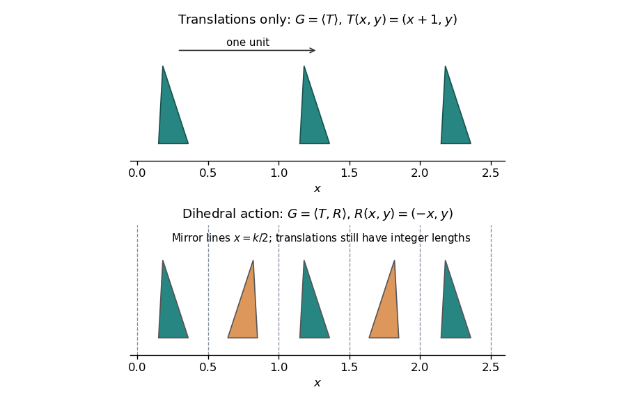
Two examples with are the group generated by alone, and the infinite dihedral group generated by together with . The latter has ; its elements are translations and reflections , whose mirror lines are . The first group preserves the orientation of every translated motif; the second also reverses it across these mirrors.
Shannon-Fano coding orders symbols by decreasing probability and recursively splits each consecutive block into two groups with probability totals as close as possible, appending bits zero and one. Huffman coding instead repeatedly merges the two least probable nodes, constructs a binary tree upwards, and then assigns the branch bits. Both yield prefix codes, so a concatenation can be decoded without separators; Huffman coding minimizes expected length among binary prefix codes.
For the specified probabilities, the first Shannon-Fano coding split is of mass versus the remaining mass . Split the latter into of mass and of mass , and then split off . One resulting code isIts expected word length is .
The Huffman coding merges are , , , and . Reading the resulting tree gives the same code lengths , and it may give exactly the displayed code if the branch bits are chosen accordingly. Its expected length is also bits. The methods agree here; their agreement on this particular distribution is not a claim that the two procedures always coincide.
Differentiate the normalization of the exponential family density with respect to , assuming the regularity that permits differentiation under its integral. The density derivative is . ConsequentlyDifferentiating the expectation once more gives , soThe log-likelihood derivative with respect to is . For the generalized linear model with linear predictor , the chain rule givesUsing independence to add the log-likelihood contributions proves the score functionHere includes the dispersion parameter . Defining instead a unit-dispersion variance function would require retaining an explicit in the denominator.
The nullclines are and , both decreasing curves in the positive quadrant. To their left/right the horizontal velocity is respectively positive/negative; below/above the second nullcline the vertical velocity is positive/negative. Bounded positive synthesis functions give an inward-pointing sufficiently large rectangle, while the axes point into the quadrant. More directly, put : , and for large enough . Continuity therefore gives a positive equilibrium.
At an equilibrium, the Jacobian matrix is , with eigenvalues . Its logarithmic-slope product isbecause and . Thus a product exceeding one makes this equilibrium a saddle and gives . Immediately on its left , and immediately on its right . Since and is eventually negative, there must be other roots on both sides, crossing in the attracting direction. For simple roots those have , hence two negative Jacobian eigenvalues: the saddle separates at least two stable steady-state alternatives. The divergence is , so periodic attractors cannot replace these equilibria in a bounded planar region. Nongeneric flat crossings or intervals of equilibria require a nonlinear stability interpretation; the strict saddle inequality alone does not guarantee that every other root is hyperbolic. This is the usual mutual repression stability criterion behind bistability.
The conclusion also has a nonlinear trapping justification. Choose on the left of the saddle with ; such endpoints exist by the signs just proved. The rectangle is forward invariant: on the vertical edges, and , while the horizontal-edge velocities point inward or are tangent. The same construction on the right of the saddle gives a second disjoint trapping rectangle. Each contains a nonempty compact attracting invariant set, obtained by intersecting its nested forward images; strict vertical inwardness also rules out invariant boundary trajectories. If a downward crossing is isolated, endpoints can be taken arbitrarily close to it, proving nonlinear stability, and the absence of periodic orbits makes nearby trajectories converge to that equilibrium. Intervals of equilibria instead give attracting alternatives consisting of families, so bounded monotone functions without nondegeneracy do not necessarily produce two isolated hyperbolic attractors.
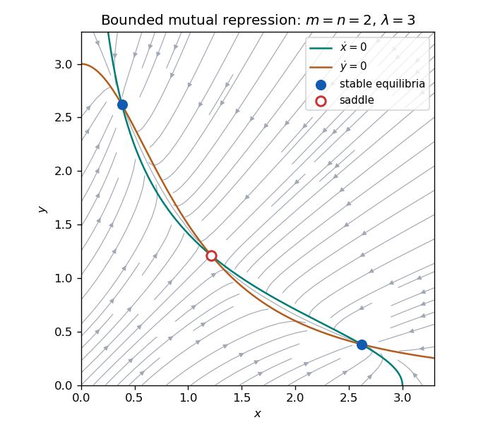
Nullclines, flow directions and two stable equilibria separated by a saddle in a bounded mutual-repression model
. Details. At a positive equilibrium of the bounded Hill model, the mutual repression stability criterion becomesThus is necessary. Because the same is imposed in both synthesis functions, it is not sufficient for arbitrary unequal positive exponents. The additional equilibrium constraint isHere is an exact criterion for all the printed exponent choices, including nonintegers. If and , multistability is possible: for large the intermediate equilibrium satisfies , , so both increase without bound and . These asymptotics follow by balancing and ; the limiting two algebraic equations have a nonsingular log-Jacobian when , so a nearby exact equilibrium exists for large . If both exponents are at most one, everywhere and multistability is impossible.
For the remaining case, interchange if necessary so . For each , let be the unique solution ofwhich exists because the left side is strictly decreasing; for the right side always exceeds one. DefineThen the exact answer for this remaining range isThis is a one-variable test depending only on , with no unknown . To prove it, parameterize all equilibria by . Implicit differentiation givesThe denominator is positive, and goes from zero to infinity as goes from zero to infinity. A negative-slope portion therefore forces two folds and an interval of three equilibria, with two attracting branches. If everywhere, is strictly increasing apart from possible isolated stationary points, so there is only one equilibrium for each . This is the common-strength Hill repression criterion.
For illustration and a closed test on the boundary , andobtained at . In particular has but maximum , so it cannot be multistable. For positive integer exponents the allowed choices simplify to both exponents at least two, or one equal to one and the other at least four. For arbitrary real exponents the preceding exact criterion is needed; replacing it by would discard the common-strength constraint.
The unbounded power laws behave differently. Combining their equilibrium equations gives . If , there is exactly one positive equilibrium,Its slope product is exactly , so it is attracting if and a saddle if , but there are never two isolated attracting equilibria. If , equilibria exist only when ; when this holds there is a whole curve of equilibria, with a zero tangent eigenvalue and transverse eigenvalue . This includes , , for every . A neutrally degenerate continuum is not bistability between isolated attractors. Thus these power laws do not generate ordinary multistability; boundedness was essential to the outer-root argument in part (a).
The Bendixson-Dulac criterion says that if a planar field admits a multiplier on a simply connected region such that has one strict sign there, no nonconstant periodic orbit lies wholly in that region. The Poincaré-Bendixson theorem says that a nonempty compact omega-limit set of a planar flow which contains no equilibria is a periodic orbit.
For , the divergence of the given field is throughout the plane. Taking proves there are no periodic orbits.
For , use . Along trajectories,On a circle with the radial flow is outward or tangent, and on a circle with it is inward or tangent. Their intervening closed annulus is positively invariant. At the tangent points , the field has , so no equilibrium sits on its boundaries. Indeed the only equilibrium is the origin, excluded from the annulus. Every forward trajectory in the annulus has a nonempty compact omega-limit set without equilibria. The Poincaré-Bendixson theorem consequently proves at least one periodic orbit exists for every . No claim of uniqueness follows from this trapping argument.
A Papperitz symbol records the three regular singular points of a second-order Fuchsian differential equation and the two local exponents at each. Exponents at infinity refer to solutions behaving as , that is, to powers of the local coordinate . Their sum satisfies the Fuchs relation: the six exponents add to one. The symbol represents the two-dimensional solution space, not one normalized solution by itself.
The specified exponents give the Gauss hypergeometric equationSet and let . Its equation isFor , differentiation gives and . Substitution into the first equation leaves times exactly the second equation: its coefficient is , and its coefficient simplifies to . Hence solves the same equation as .
The symbol gives the same check geometrically: multiplication by shifts the exponents at one from to and those at infinity from to ; it does not change the exponents at zero. Choose the branch with . Then is analytic at zero and . For the analytic recurrence uniquely determines this normalized solution, provingThe identity continues wherever both sides are defined with compatible branches. At exceptional parameters where the stated normalization does not uniquely define an analytic function, a parameter-continuation convention is needed; the generic proof does not silently assume uniqueness there. This is Euler's hypergeometric transformation.
There are two degrees of freedom, conveniently the azimuthal angles on the two circles. The positions are and . Their squared separation is . Thus the Lagrangian isThe constant terms may be omitted from the equations of motion. In this notation is the stated spring coefficient, with the units needed for potential energy; it is not automatically an angular frequency for arbitrary masses.
For dilute nonrelativistic nucleons in thermal equilibrium, their Maxwell-Boltzmann distribution gives . The neutron and proton spin degeneracies are equal, and their mass prefactor ratio is nearly one. ThusWeak reaction equilibrium imposes . Charge neutrality in an electron-positron plasma, together with the small baryon asymmetry, makes very small. Assuming negligible neutrino lepton asymmetry also makes small. Hence the difference, rather than the absolute baryon chemical potentials, is negligible, yieldingA large neutrino chemical potential would invalidate this last approximation; it is an assumption about the lepton asymmetry, not a general rule that baryonic chemical potentials vanish.
The weak-conversion rate per expansion time falls as . Below the stated threshold it becomes less than one, so neutron-proton interconversion cannot track the rapidly changing equilibrium ratio: cosmological weak freeze-out occurs. Free neutrons subsequently decay, reducing their abundance until nuclei can survive photodissociation. Once the deuterium bottleneck is passed, nuclear reactions rapidly assemble neutrons into the strongly bound helium-4 nucleus. The short available time, low density and missing stable mass-five and mass-eight nuclei impede extensive production of heavier nuclei, leaving nearly all surviving neutrons in helium.
If just before helium formation, each helium nucleus uses two neutrons and two protons, so . Neglecting binding-energy corrections to nuclear masses,The remaining protons mainly become hydrogen. Counting all four helium nucleons, rather than only the captured neutrons, is essential to this mass fraction.
If the weak-rate coefficient is reduced, equality with the expansion rate occurs at a higher temperature, since scales as that coefficient times . The freeze-out temperature and interaction strength relation is . The frozen neutron-to-proton ratio is then closer to one, so the primordial helium mass fraction increases, potentially approaching unity if nearly equal numbers survive to nucleosynthesis. If the same weaker interaction also slows free-neutron decay, it reinforces this trend; changing conversion rates alone would instead require a separate treatment of the decay interval.
Less primordial hydrogen means less hydrogen fuel and, for otherwise comparable stellar physics, helium enrichment raises the mean molecular weight, tending to make a fixed-mass star hotter and more luminous and to shorten its hydrogen-burning lifetime. A genuinely weaker weak interaction also changes proton-proton fusion itself, so a quantitative lifetime cannot be inferred from composition alone. Much less hydrogen and fewer long-lived suitable stars would alter planet formation, water availability and the timescales needed for life on Earth. These are physical implications of the changed initial composition, not a numerical prediction of habitability from the helium fraction alone.
The triangular-grid form is Sperner's lemma: subdivide a triangle into small triangles meeting edge to edge, label its vertices , and forbid label on the side opposite corner . The corner labels are thereby forced. An odd number of small triangles, in particular at least one, carry all three labels.
Here is the parity proof. Count incidences of a small triangle with an edge whose endpoint labels are . On the outer boundary these edges occur only on the side joining corners ; traversing that side begins with label one and ends with label two, so the number of changes of label is odd. Interior edges contribute twice to the incidence count. A small triangle with all three labels contributes once; a triangle having only labels one and two contributes twice if it has both, and all other triangles contribute zero. Reduction modulo two therefore proves the assertion.
To obtain the continuous Brouwer fixed-point theorem on the triangle, use barycentric coordinates and a continuous map from the triangle to itself. If a grid vertex is not already fixed, label it by an index with , which exists since both coordinate sums are one. A point on the side cannot receive label , so the discrete lemma applies. On successively finer grids take a fully labelled small triangle. Compactness gives a subsequence converging to one point ; all three vertices converge to it because the mesh tends to zero. Passing to the limit in the three label inequalities gives for every . Equal coordinate sums force equality throughout, hence .
A closed disk is homeomorphic to a triangle: radial coordinates from an interior point, scaled by the distance to the boundary in each direction, give such a homeomorphism. Conjugation therefore gives the same fixed-point assertion on the disk. If were a continuous retraction from the unit disk to its boundary, define . A fixed point would have , hence and , impossible on the unit circle. Thus no continuous disk-to-boundary retraction exists. The continuous conclusion has been deduced from the grid parity argument, not used to prove it.
In the hyperbolic-ball model, the limit set of a Kleinian group is the boundary accumulation set of an orbit of an interior point: . The choice of does not matter, since any two such orbits remain a fixed hyperbolic distance apart. It is closed and -invariant. The complicated/non-elementary hypothesis excludes relatively compact groups and elementary groups with at most two limit points; in particular the limit set is nonempty. Having no finite boundary orbit alone would not exclude a compact rotation group, whose interior orbits are bounded.
If were finite and nonempty, the orbit of any of its points would be a finite boundary orbit, contrary to the hypothesis. Thus it is infinite. In fact it cannot be countable. We give the essential minimality/perfectness argument. A sequence of Möbius transformations sending an interior point toward has a subsequence converging on the boundary away from one exceptional point to the constant . This follows by normalizing the representing matrices: a diverging sequence has a rank-one projective limit, with one kernel line and one image line. For any boundary point , the absence of a finite orbit allows choosing with different from that exceptional point; then . Hence the orbit of every is dense in .
If were an isolated limit point, density of every orbit would make every point belong to its orbit: each orbit must hit the open singleton . Every point would then be isolated by equivariance, making the compact set discrete and therefore finite, a contradiction. Thus is a nonempty perfect compact metric space. Repeatedly choosing two disjoint smaller neighbourhoods meeting this perfect set, with diameters tending to zero, associates distinct nested limits to all infinite binary sequences. The limit set is therefore uncountable.
Jorgensen inequality states that for a non-elementary discrete group generated by lifts ,For a concrete failure of discreteness, take and with small. The fixed points of and of collectively include , so the group is non-elementary. Direct multiplication gives both summands equal to . Their sum is less than one when is sufficiently small, proving this two-generator group is not discrete.
For a connected-limit-set example, the modular group generated by and is discrete because its matrices have integer entries. It preserves the upper half-plane; its limit set is the extended real line, a circle. Indeed the orbit of the parabolic fixed point infinity consists of the rational points and infinity, dense in that circle. For a disconnected example, choose four pairwise disjoint round disks and two loxodromic maps pairing the exterior of each negative disk with the interior of its positive disk. The Schottky group generated by these maps is free and discrete by the disjoint-domain ping-pong construction. Successive reduced words give nested disjoint disks with shrinking diameters; their limiting points form a Cantor set. Thus its limit set is disconnected, unlike that of the modular group.
The data are read row by row into a vector of 84 prices. The first factor cycles through the six goods within each row; the second repeats each of the fourteen resort levels for six entries. Thus the linear regression fits one observation per resort-good cell, after taking natural logarithms. With treatment coding, its underlying statistical model isfor resorts and goods . This is an additive two-way analysis of variance on log prices, equivalently a multiplicative resort/goods model on the price scale, with no interaction. There are fitted parameters and .
In a balanced complete table, the fitted log price is the resort row mean plus the goods column mean minus the grand mean. Thus every resort coefficient is its row mean minus the Algarve row mean, and every goods coefficient is its column mean minus the meal column mean. The intercept is the fitted mean log price for a meal in Algarve, not necessarily the observed log price in that cell. Exponentiating coefficients gives price multipliers: the beer coefficient corresponds to approximately times the meal scale, and car hire to times that scale. Likewise the Sorrento resort effect gives a common factor relative to Algarve, if the no-interaction model is valid.
The standard errors are computed from with . Balance gives goods-contrast standard error and resort-contrast standard error . Each reported t statistic is its estimated coefficient divided by its standard error. Under the Gaussian model and the corresponding zero-coefficient null, it has a Student t-distribution with 65 degrees of freedom; the reported probabilities are two-sided tail probabilities. All goods contrasts are strongly significant, largely reflecting unlike goods and units of purchase. Among the resort contrasts, Costa del Sol, Majorca, Florida, Sorrento, Sicily and Madeira have unadjusted probabilities below . This is six separate comparisons with Algarve, not a simultaneous ranking guarantee or an omnibus test of all resorts. Multiple comparisons and model adequacy must be considered before declaring a universal cheapest resort.
The residual standard error measures variation on the log scale; is a typical multiplicative one-standard-deviation factor. Under the lognormal distribution, estimates the conditional median/geometric mean price, while the arithmetic mean has the additional factor . The reported means 96.2 percent of the observed log-price sum of squares around its overall mean is explained. It does not mean resorts alone explain that fraction, nor that 96.2 percent of variation on the original price scale is explained.
With only one observation per cell, unrestricted goods-by-resort interactions cannot be estimated separately from residual error. The model assumes comparable quoted items, approximately common log-error variance, independent errors and common resort multipliers across goods. Residuals can reveal failures, such as a particular resort having unusually costly taxis but ordinary prices for other goods. The intercept's test against zero concerns a fitted baseline geometric price of one pound; it is not an assessment of the overall model's validity.
At a fixed point , and the first equation factors. The branches areThe three branches meet at , and the positive square-root branch meets the quadratic branch at . The Jacobian matrix at a general fixed point isOn , its trace is and determinant : the branch is attracting for and a saddle for or . On , the eigenvalues are and . The negative branch is always a saddle for ; the positive branch is a saddle for and attracting for . At the bifurcation values the zero eigenvalue requires the nonlinear analysis below.
For , , , the equations areThe extended centre manifold has with no linear terms. Since has degree at least three, its invariance equation to degree two is . ThusThe reduced quadratic factors as . Its two roots have reduced eigenvalues and , respectively, and the transverse eigenvalue remains negative. They exchange stability at , a transcritical bifurcation. The exact branches have and , consistent with this second-order evolution equation.
Near , the slow equation has leading form , so this is a subcritical pitchfork bifurcation with the parameter orientation displayed. For there is one nearby saddle, whose unstable direction is close to and stable direction close to vertical. For the central branch is attracting and the outer two equilibria near are saddles; their separatrices distinguish attraction toward the central equilibrium from departure outwards. The actual central location is , not exactly the origin away from .
Adding positive breaks the pitchfork symmetry. The leading equilibrium equation near zero is : the diagram unfolds into a single branch plus a saddle-node pair, with the latter appearing for positive of order . More precisely the fold is at , at leading order. Near one the reduced equation becomes . Its discriminant is ; the crossing is replaced by two saddle-node endpoints with a no-equilibrium gap for to leading order. Outside that gap, the lower reduced root is stable and the upper one unstable. These local approximations describe the sketch; the exact perturbed curves have higher-order corrections.
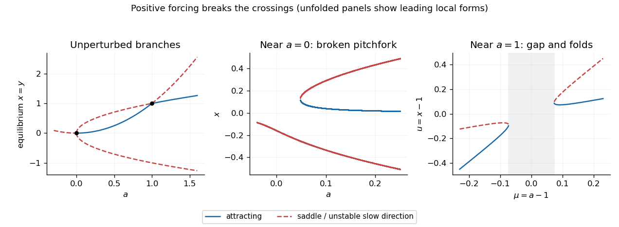
Fixed-point branches, local phase portraits and the positive-forcing unfoldings of the pitchfork and transcritical bifurcations
. Details. 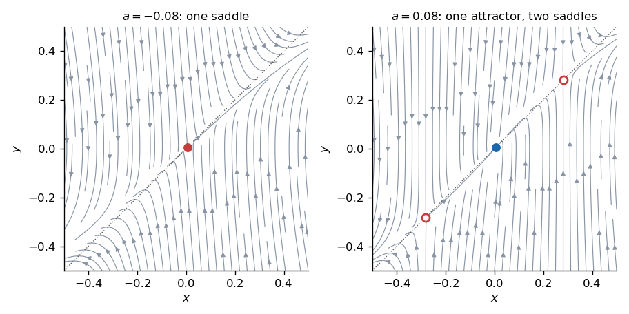


Consider a smooth variation with . Differentiating the action at zero and integrating the velocity term by parts givesThe boundary term vanishes because the endpoints are fixed. Independent compactly supported variations and the fundamental lemma of the calculus of variations make every bracket zero. Thus the Euler-Lagrange equations areThe required principle is stationarity of the action; an extremal need not be a strict minimum.
Measure from the downward vertical, so the bob is at . Its squared speed is . Up to a constant potential term, the Lagrangian isThe Euler-Lagrange equations giveAt the downward stable equilibrium, linearization gives and . Eliminating yieldsThere is also a zero-frequency translational mode because the rail fixes no preferred pivot position.
If an external force imposes constantly, the bob's angular equation becomes . Its stable equilibrium therefore hason the branch near the downward vertical. The displaced bob leans opposite the acceleration. The solution differing by is unstable, corresponding to alignment opposite the effective gravitational field in the accelerating frame.
Zorn lemma states that a nonempty partially ordered set in which every chain has an upper bound contains a maximal element. To prove it from the axiom of choice and Hartogs theorem, suppose no element were maximal. Fix a choice function on the nonempty subsets of the poset. Every chain then has a strict upper bound: choose an upper bound, and, since it is not maximal, choose an element strictly above it. Let be a Hartogs ordinal which cannot inject into the poset. By transfinite recursion for , choose a strict upper bound of all previously chosen , ; for the empty initial chain choose any element. The previous elements form a chain at every stage. The resulting strictly increasing sequence injects into the poset, contradicting Hartogs. Hence a maximal element exists. Choice is used in fixing the function selecting a strict upper bound at every successor and limit stage; Hartogs and transfinite recursion themselves do not supply those selections.
Apply Zorn lemma to the linearly independent subsets of over , ordered by inclusion. A chain's union is linearly independent because any finite linear relation is contained in one member of the chain. A maximal independent set must span , since otherwise one could append a vector outside its span. Thus is a rational-vector-space basis of .
It is infinite: a finite-dimensional rational vector space is countable, whereas is not. If its cardinal is , finite rational linear combinations show ; uncountability forces . A basis of is , where these expressions mean the vectors and . Its cardinal is , using the infinite-cardinal arithmetic available under choice. A bijection between the two bases extends uniquely by finite rational linear combinations to a linear bijection. ThereforeThis is an algebraic isomorphism, with no assertion of continuity or real-linearity.
For the first assertion, use the standard nonempty finite-graph convention. Choose a longest simple path in an acyclic graph. Its endpoint can have no neighbour outside the path, or the path could be extended; it can have no neighbour farther back than the adjacent path vertex, or there would be a cycle. Its degree is therefore at most one. The qualification matters for infinite graphs: a two-sided infinite path is acyclic and every vertex has degree two.
A finite tree with has a leaf by this argument and connectedness. Removing it and its one edge leaves a tree with vertices. Induction from the one-vertex tree proves a tree of order has edges. Conversely, a finite connected graph has a spanning tree: begin with one vertex and repeatedly add an edge to a new vertex until every vertex is reached. This creates no cycle and uses edges. If the original graph has exactly that many edges, it equals its spanning tree and is itself a tree.
To embed a tree of order , root it and list its vertices so every nonroot vertex follows its parent. Embed the root at any vertex of . When embedding a new vertex, at most neighbours of its parent's image are already used, while that image has degree at least . An unused neighbour exists and can be chosen. This constructs an injective edge-preserving copy of , soFor , the complete graph has minimum degree but too few vertices to contain . Thus the degree bound cannot be lowered in general. A subgraph copy need not be induced; extra edges in do not obstruct the construction.
An element of an extension is an algebraic element over when some nonzero polynomial in vanishes at . Let its monic minimal polynomial have degree . Polynomial division shows is spanned by , and minimality makes these vectors independent. The minimal polynomial is irreducible; for any nonzero , Bezout's identity between and that polynomial gives a polynomial representative for . Thus is a field, equals , and has degree .
Conversely, if has finite vector-space dimension , then are linearly dependent over , giving a nonzero annihilating polynomial. HenceAn algebraic extension is one in which every element is algebraic. Suppose and are algebraic, and take . A polynomial relation for over uses only finitely many coefficients . Each is algebraic over , so adjoining them successively gives a finite extension , by the proved criterion and the tower law. The same relation makes algebraic over , so is finite. Therefore is finite, and its subspace is finite-dimensional. The criterion makes algebraic over . Since was arbitrary, is algebraic.
The character of a permutation representation at equals the number of points fixed by , because a permuted basis vector contributes one to the trace exactly when it is fixed. Thus the character inner product isTo identify the last average, count pairs with . Each orbit contributes , since its number of elements times their common stabilizer size is by the orbit-stabilizer theorem. ThereforeThe conjugation in the usual character inner product has no effect here because the permutation characters are real-valued.
There is a missing hypothesis in the printed equivalence. A group acting trivially on a two-point set has a one-dimensional zero-sum subspace , hence an irreducible trivial representation, but its action is not doubly transitive. Thus the assertion as written is false. The intended result holds for a transitive action; more generally the trivial two-point action is the only exceptional case under .
For the intended proof, decompose by separating constant functions from functions with zero sum. If the action is transitive, . HenceOver the complex numbers, complete reducibility and character orthogonality identify this norm as the sum of squared irreducible multiplicities; it is one precisely when is irreducible. By part (i), counts orbits on . Transitivity gives one diagonal orbit, and the norm equals two exactly when all off-diagonal ordered pairs form one orbit, which is double transitivity. This proves both implications with the missing transitivity condition restored.
To check the exact exception, if the action has orbits, then contains an invariant subspace of dimension , from orbitwise constant functions with total sum zero. If is irreducible this makes the one-dimensional trivial representation, so and . Nontransitivity on two points means both are fixed. Therefore irreducibility is equivalent to double transitivity, except for the trivial two-point action.
The symmetric group is transitive on two-element subsets, giving . Its diagonal action on has two orbits, according to whether the point lies in the pair. Thus , and, since , the standard zero-sum representation occurs in once. Its irreducibility follows from the double transitivity of the natural symmetric-group action and the corrected statement of part (ii).
For , ordered pairs of two-element subsets have three possible intersection sizes, zero, one and two, each forming a single orbit. Part (i) therefore gives . After removing the one copy each of and , the remaining character has squared norm , so is itself irreducible. HenceFor , taking the complement of a pair is an equivariant bijection . Thus , with no third constituent. Correspondingly the disjoint-pair orbit is absent and the character norm is two.
The three quadratic subfields are , and . Their integer rings are respectively , and , since their squarefree radicands are modulo four. Write . Relative traces to these three fields are , and . Traces of algebraic integers are integral, so all four doubled coefficients are integers. ThusThe PDF names the wrong quadratic subfield for its next displayed norm coefficients. They are obtained from , not . The relevant conjugation changes the sign of , givingIts membership in proves the requested divisibilities. For comparison, the norm to the printed subfield is , a different expression.
The first divisibility modulo two makes have the same parity. The second makes even, so they cannot both be odd: and are even. Substituting this into the first divisibility modulo four shows is even, hence . Therefore every algebraic integer is an integer linear combination ofIndeed the last two half-coefficients are . These four elements are rationally independent. They are all integral: for , , and consequentlyis a monic polynomial with integer coefficients. Their integer span consists of algebraic integers and contains every algebraic integer by the preceding argument, proving the integral basis of a two-prime biquadratic field. This repairs the subfield typo without changing the claimed basis.
The assertion needs connected. Without that assumption, the disjoint union of two tori mapping by the identity on each component is a covering of the torus and is none of the three listed connected spaces. The correct general statement classifies each connected component; here is the intended connected proof.
The universal cover is , and . The classification of connected coverings of a connected, locally path-connected, semilocally simply connected space identifies with for a subgroup , acting by translations. A subgroup of is free abelian of rank zero, one or two. For rank zero the quotient is the plane. For rank one, a linear coordinate change sends its generator to a translation in one coordinate, yielding . For rank two, a linear coordinate change sends a lattice basis to the standard basis, yielding a torus. Thus a connected covering is a plane, cylinder or torus. For arbitrary , its covering components are disjoint unions of these types, rather than necessarily one such space.
For , the sphere is simply connected. The lifting criterion for a covering space says that a based map lifts to a covering whenever the image of its fundamental group lies in the subgroup corresponding to that covering. For the universal cover , the sphere's trivial fundamental group meets this condition. Hence has a continuous lift .
Contract the lift linearly to any point :This is a continuous homotopy from to the constant map . Thus every such sphere-to-torus map is null-homotopic. The restriction is essential; circle maps may carry nonzero fundamental-group classes.
In the supremum-norm metric, is totally bounded if for every finitely many norm balls of radius cover it. It is uniformly bounded if some satisfies for all . It is equicontinuous if for each and there is a neighbourhood of with for all . This definition works for compact Hausdorff without assuming it is metrizable.
Suppose is totally bounded. A finite radius-one net makes uniformly bounded by one plus the largest norm of a net centre. For equicontinuity, choose a finite net. Continuity of each centre gives a common neighbourhood of on which all centre values vary by less than . Approximating any by its centre and using the triangle inequality at and bounds its variation by . Thus both conditions follow.
Conversely suppose those two conditions hold. For each , choose a neighbourhood on which every function varies from its value at by less than . Compactness provides a finite cover . The vectors form a bounded subset of , so partition their possible values into finitely many boxes of diameter less than in the maximum-coordinate norm. From each occupied box choose one function as a representative. If and its representative have sample values in the same box, and , thenThese finitely many representatives are a norm net, proving total boundedness is equivalent to uniform boundedness and equicontinuity. This supplies the finite-net part of the Arzelà-Ascoli theorem directly.
For a bounded set that is not totally bounded, take the standard unit vectors in the Banach space . Their norms are one and their pairwise distances are . A ball of radius less than contains at most one of them, so finitely many such balls cannot cover .
The local estimate gives at zero and, by periodicity, at every lattice point. If two candidates existed, their difference would extend to an entire doubly periodic function: the principal parts cancel at every possible pole. It is bounded on a fundamental parallelogram, hence on the plane, so Liouville theorem makes it constant. The local difference tends to zero, making the constant zero. Thus the function is unique.
The function has the same periodicity, poles and local estimate. Uniqueness therefore proves . Its Laurent expansion is consequentlywith no constant term by the given estimate. Periodicity and evenness imply , so . The elliptic zero-pole counting theorem says a nonconstant elliptic function has, in one period cell, equally many zeros and poles counted with multiplicity. Applied to , whose total pole order is two, it gives precisely two zeros counted with multiplicity. The zero at already has multiplicity at least two. It therefore has exactly two, provingFinally is periodic, and the Laurent expansion shows cancellation of all possible pole terms: and . The difference extends to an entire bounded function and is constant. HenceEvery property of the Weierstrass elliptic function used here has been obtained from the stated local and periodic properties, together with the explicitly stated standard elliptic-function counting theorem.
A point is a critical point of a smooth map if is not surjective. A critical value is the image of at least one critical point. A regular value is a point for which every point of has surjective differential. A point outside the image is therefore a regular value vacuously. These definitions use rank relative to , not merely whether a derivative vanishes in chosen coordinates.
Let , , and . In coordinate charts centered at and , write the map as . Surjectivity of its derivative gives an invertible minor; reorder the domain coordinates so it is the first one. The maphas invertible derivative at the point. By the inverse function theorem, it is a local coordinate change. In these coordinates the fiber is simply the set whose first coordinates are zero, so it is locally a coordinate plane of dimension . These charts are inherited from , provingIf the fiber is empty, it is the empty submanifold under the usual convention. The no-boundary assumptions avoid any extra boundary conditions in this local model.
Regard the space of real matrices as , and use the smooth determinant map. For invertible , factor . Expanding the determinant to first order givessince the linear coefficient of is the sum of the diagonal entries of . At every with determinant one, taking makes this derivative . Thus one is a regular value, and part (ii) makes a submanifold of dimension .
Its tangent space is the kernel of this differential. At the identity,Indeed tangent derivatives of curves with constant determinant lie in that kernel, and the local regular-value coordinates show every kernel vector is tangent to the level set.
A pi-system is a collection closed under finite intersections. The uniqueness theorem says that two probability measures agreeing on a generating pi-system agree on its generated sigma-field. For finite measures one also fixes the total mass; for a sigma-finite version one requires a covering sequence from the pi-system with finite common masses. Adding the whole space to a pi-system of events causes no change to its generated sigma-field and preserves the stated independence condition.
Fix . On the finite measures and agree on and on the whole space. Uniqueness makes them agree for every . Now fix such an . On the measures and agree on and the whole space; a second application of uniqueness provesThus the two generated sigma-fields are independent. The extension is done one argument at a time, not by assuming the required independence for arbitrary unions.
For the independent random variables, let be the rectangles and let be the analogous rectangles in the . Both are pi-systems. Joint independence of the full list factors each combined rectangular probability into the product of the individual probabilities, hence into . Their generated sigma-fields are exactly and . The proved result therefore gives independence of the two vector-generated sigma-fields.
Let , with finite offspring mean . Conditioning on the original cell's first exponential lifetime givesEach of its offspring starts an independent copy of the process, which explains the factor . Changing to and differentiating yields , . HenceFinite-mean truncation and this integral bound justify finite expectations and exclude explosion in finite time; it is not necessary to assume a bounded offspring count.
For the probability generating function, let . Independence of offspring populations gives the conditional generating function at a first division time. Thusand differentiation of the changed-variable integral provesFor , the integrand is bounded, so this generating-function argument has the needed convergence even without higher offspring moments.
With two offspring always, the backward equation becomes . Separation and the initial value giveThus is geometric on the positive integers, andThis is a Yule process shifted down by one. It is not an inhomogeneous Poisson process. Given , its instantaneous jump rate is , a state-dependent random rate rather than a deterministic function of time. Also whereas , unequal to the mean for . Its mean arrival intensity does not turn its dependent increments and geometric marginals into Poisson ones.
Wilks theorem states that, under an interior null parameter and the usual identifiability, smoothness and nonsingular-information regularity conditions, for nested models converges under the null to a chi-square distribution with degrees of freedom equal to the difference of parameter dimensions. Boundary or nonidentifiable nulls need not have this distribution.
Write , and . The unrestricted maximum-likelihood estimates are and . Under the null the variance estimate is . Substituting both maxima into the Gaussian likelihood givesThis is for , with positive true variance; almost surely. The lost parameter dimension is one, even though variance is estimated in both models.
The two-sided Student t-test uses , where , and rejects when . Under the null has exactly the Student t-distribution with degrees of freedom. The likelihood-ratio statistic isunder the null, so its chi-square approximation agrees asymptotically with the squared asymptotic standard-normal t statistic. In fact the expression is strictly increasing in : with exact finite-sample calibration the tests have identical rejection regions for every , not just approximately for large samples.
The reservation bid price for a claim is the fixed cash payment which leaves the agent indifferent: . For Gaussian wealth , exponential utility is , so its certainty equivalent is . For , subtracting the original certainty equivalent givesThe marginal price is positive when the claim hedges the agent's endowment, negative when it adds positively correlated risk, and zero for an uncorrelated zero-mean infinitesimal position.
Assume , so the claim is nontrivial. Buying units at per-unit price changes the certainty equivalent by . This strictly concave quadratic is maximized at . Market clearing givesAt the optimum the certainty-equivalent gain isThe maximal expected utility equals the original negative utility multiplied by , hence is improved. Paying a fixed amount removes exactly that gain, proving it is the fixed-payment value of market access. If , the Gaussian claim vanishes almost surely, all its covariances vanish, and the appropriate price and access value are zero; the printed formulas with a variance denominator require the nontrivial-claim assumption.
For a regular defining function , the hypersurface is non-characteristic when the characteristic vector has nonzero normal component:For this is precisely . The defining function must also have nonzero gradient so that it actually defines a hypersurface.
The method of characteristics gives , , , . Starting at , the first two coordinates rotate clockwise through characteristic time and . Solving back for the initial point givesIt meets the data and is when is .
For the rotationally invariant data, . As it tends to zero for fixed , diverges to positive infinity for fixed and nonzero radius, and retains the initial value on . It is identically zero on the vertical axis. There is no regular limit across the initial plane. At that plane is characteristic and the data would need to satisfy ; the chosen radial data violate this except at the origin, explaining the singular limit.
An asymptotic power series about means that for every fixed ,as through the specified domain. It makes no assertion that the infinite series converges at nonzero . If a power series converges in a neighbourhood, choose a smaller fixed convergence radius : absolute convergence bounds its tail after by for . Thus a convergent power series is also asymptotic. The coefficients are unique, successively recovered byIf two expansions first differed at index , division of their difference by would contradict this limit.
For the given integral, use the exact finite identity . The gamma integral givesConsequentlyFor the denominator is at least one, soThe empty product for is one. The bound is exactly the magnitude of the next omitted term. For the asymptotic definition through degree , take , giving an remainder. Only a finite expansion was integrated; interchanging a divergent infinite series with the integral would be invalid. Indeed the ratio of consecutive term magnitudes is , so this formal series diverges at every fixed .
Let , with interior and exterior boundary values . The Sokhotski–Plemelj formula gives and . Write for the nonlocal scalar moment. Substitution into the integral equation yieldsThus the associated scalar Riemann-Hilbert problem isThe functions are analytic in their respective interior/exterior domains, and must ultimately equal the moment of the recovered jump; it is not an independently specified free constant.
The jump coefficient has one enclosed pole at zero and no enclosed zeros, because are outside. Its winding index is therefore . A homogeneous canonical pair isEach is analytic and nonvanishing in its required finite domain; the exterior growth encodes the negative index. Dividing the unknown by these factors gives an additive jumpThe Cauchy-integral solution for normally has an exterior coefficient . Since must decay, this coefficient must vanish. Thus the solvability condition is . Its only enclosed pole is zero, with residue , soThese are the negative-index scalar Riemann-Hilbert moment conditions for index minus one. There is no arbitrary polynomial addition: an entire addition respecting is zero by Liouville's theorem.
With , the additive jump is , analytic inside the contour. Its Cauchy integral has and . Therefore , , andThe moment is indeed , as required. The principal-value Cauchy sum is , and the original left side becomes . Thus the recovered function satisfies both the equation and the self-consistency condition, and the homogeneous negative-index argument proves uniqueness.
The commutator gives . Hence and . Starting with the normalized vacuum, repeated application gives , proving unit norm. The number operator then has eigenvalue , soDifferent levels are orthogonal because the Hamiltonian is self-adjoint and their eigenvalues are distinct.
For the perturbation, the ground-state diagonal matrix element is zero, while . The nondegenerate second-order perturbation formula consequently givesFor , . The lower and upper intermediate levels contribute respectively and , giving to second order.
For the exact completion of the square isThe shifted operators , have the same commutator and are unitarily related to the original ones by a displacement operator. Their vacuum is the coherent state with amplitude . Therefore every exact level shifts by .
The stability of monomial ladder-operator perturbations gives a necessary qualification to the request for a lowest level for every . For and real nonzero , a coherent state of amplitude has energy expectation . Choose the phase so the last term is negative. As the expectation tends to minus infinity, so the perturbed Hamiltonian has no true ground state. The displayed second-order answer is then the formal perturbative coefficient of the branch from the unperturbed vacuum, not an exact lowest eigenvalue. For stability requires ; for the completed-square Hamiltonian is bounded below for every real .
The differential scattering cross-section is scattered rate per unit solid angle divided by incident flux. For the outgoing scattering solution, the incident plane wave has current magnitude , while the outgoing spherical wave has radial current . ThereforeThe incoming plane-wave normalization and outgoing radiation condition select the physical scattering state.
The time-independent Schrödinger equation is , equivalently . The given outgoing Helmholtz fundamental solution has source . Multiplying it by the source and adding the incident homogeneous solution givesApplying verifies its equation and sign. At large , and over the potential's support. ConsequentlyThe Born approximation replaces by the incident wave, givingIt requires weak wave distortion. A sufficient smallness condition from the integral equation is ; for a bounded potential of range this is of order . At high energy a small accumulated phase and weak deflection can also justify the approximation, but small potential relative to energy alone is not sufficient for an arbitrarily long interaction range.
For the exponentially screened potential, angular integration in its Fourier transform givesIt is not compactly supported, but for its decay gives the same scattering asymptotics and convergent integrals. Since ,Thus the Born amplitude in this limit is independent of when expressed using and angle; its squared magnitude is the Rutherford cross-section. This is a fixed-nonzero-angle limit of the Born formula. It does not establish uniform validity in the forward direction or preserve the short-range outgoing-wave asymptotics for the unscreened Coulomb potential.
Articles were limited to the first 100 out of 547 total.
Articles by others on the same topic
There are currently no matching articles.