The Chinese remainder theorem says that for pairwise coprime positive moduli , every choice of residues determines exactly one residue class modulo . Equivalently is an isomorphism under reduction.
The first two modular congruences combine to . Reducing this expression modulo seven gives , so . Consequently all integer solutions areThe moduli are pairwise coprime, so the Chinese remainder theorem guarantees that this is the entire solution class.
Define the Lagrange interpolation polynomialsDistinct interpolation nodes ensure every denominator is nonzero and . For a polynomial of degree at most , the difference has degree at most and vanishes at distinct points, so it is zero. Integrating this Lagrange interpolation identity proves the required exact quadrature formula. This also covers , when the empty product is one and its weight is two.
Use Gaussian quadrature: choose the nodes as the roots of the degree- Legendre polynomial, which are distinct and inside . Retain the integrated Lagrange interpolation weights. With the standard normalization , they can be writtenThe orthogonality of the Legendre polynomial against all lower-degree polynomials makes this quadrature exact up to degree , twice the arbitrary-node degree apart from the endpoint count. This is the Gauss–Legendre choice of Gaussian quadrature nodes and weights.
For the unit sphere, project from its north pole onto the equatorial plane, identified with the complex plane. The line through and meets the plane at the stereographic projectionThe north pole is omitted from the plane chart; adding its image infinity gives the Riemann sphere.
For a point whose image and antipodal image are finite, stereographic projection of gives . Thereforeusing . Conversely implies . Substituting this into the inverse stereographic projection changes the signs of all three coordinates, proving the converse. Thus finite chart images correspond to antipodes exactly when . On the extended chart the exceptional antipodal pair is , for which the displayed ordinary complex product is not defined.
Each test divides the current candidate set into a tested subset and its complement: failure places the defective item inside the subset, whereas success places it outside. A sequence of tests is therefore a binary decision tree, and minimizing its expected depth is the Huffman coding problem with weights .
Combine the smallest two current weights repeatedly. One choice of merges is , , , , , , , , . It gives this explicit prefix code:At any node, test the candidate items whose next code digit is one. Assign failure to digit one and success to digit zero, and repeat until only a single codeword remains. This specifies every test, including the first subset . Huffman coding minimizes the weighted codeword lengths, so the optimal expected number isThe sum of the successive merged weights is another check on the numerator .
There is a genuinely different optimal procedure. Exchange the codewords assigned to items three and four. Both have code length four, so each item's length, and hence the expected number of tests , remains unchanged. The first tested subset now contains item three instead of item four, so this changes the tested groups rather than merely reversing the names of the two test outcomes. The new prefix code still identifies every item uniquely and retains the minimum Huffman coding expectation.
The procedure in part (i) sometimes needs five tests, for items one or two. A binary decision tree of height has at most leaves, so distinguishing ten possibilities requires .
A prefix code attaining this worst-case bound isUse the same subset-testing rule. The minimum worst-case number is four, so the expected-optimal procedure is not worst-case optimal. This four-test procedure has expectation , illustrating the small cost of imposing the smaller maximum depth.
The logit link gives . Independence in the Bernoulli logistic-regression model therefore gives the log-likelihoodDifferentiate using :The maximum-likelihood estimator, if finite, solves the single score equation . If at least one is nonzero, the log likelihood is strictly concave at finite , so any root is the unique maximizer.
Use Newton method, equivalently one-parameter iteratively reweighted fitting:A damped step or a bracketed score solver is useful if a full step overshoots. The finite maximum-likelihood estimate in a one-parameter logistic model requires the score limit at minus infinity to be positive and its limit at plus infinity to be negative. Perfect sign separation of the observations can instead send the estimate to an infinite coefficient; if every , the coefficient is unidentifiable. These possibilities should be checked before claiming convergence to a finite estimate.
In the squared-denominator population map, is the low-density per-generation multiplication factor, while controls crowding: is the characteristic population scale. The nonzero fixed point for and its multiplier areSince this multiplier lies strictly between minus one and one, is locally asymptotically stable. This holds for every finite , even when the map is locally decreasing at its fixed point.
For the post-initial invariant interval for a squared-denominator population map, put and . The derivative shows that the global maximum is at . The first two iterates of the supplied initial condition are consequentlyFor , . Hence the map decreases throughout , with minimum there, and its global maximum bound ensures . Thus , and induction provesBoth endpoints are attained at . The lower bound printed without a time qualification is false at , because the given value is strictly below when . The invariant bounds apply after that initial step, not to it.
The cobweb plot below uses and . The first vertical move reaches the maximum, the next reaches its image, and subsequent vertical/horizontal steps remain in the invariant interval and approach the stable fixed point.
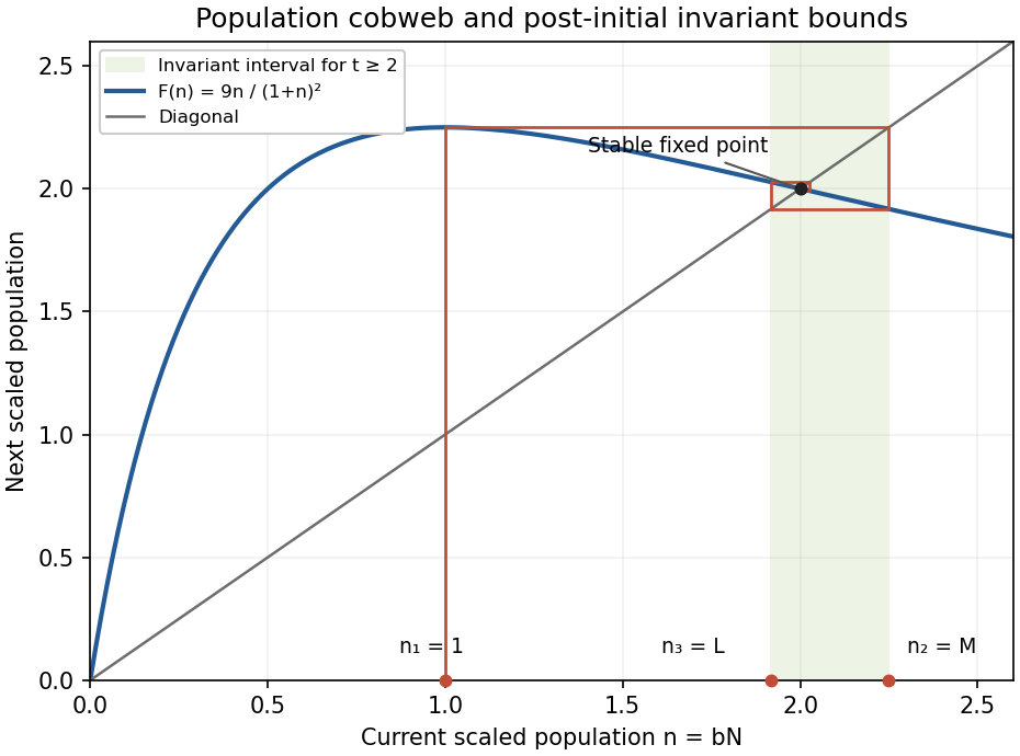
Cobweb of the squared-denominator population map, showing the invariant interval from the second iterate
. Details. 
A Lyapunov function near an equilibrium is a continuously differentiable function with , for nonzero nearby , and along trajectories there. Strict negativity away from the equilibrium gives local asymptotic stability. Lyapunov stability itself means that every prescribed small neighborhood contains a smaller neighborhood whose forward trajectories never leave the prescribed one.
For the proposed quadratic form, direct differentiation givesWhen , the quadratic part is negative definite, so it dominates the cubic remainder in a sufficiently small ball; is then a strict Lyapunov function. If , take to make the leading derivative positive. At , that same line gives , positive on its negative half. Values fail positive definiteness of . ThereforeFor the full derivative factors, with no small-amplitude truncation:Every closed sublevel set lies in , is forward invariant, and has strictly decreasing away from the origin. Compactness and the Lyapunov stability argument therefore show that the ellipse belongs to the origin's basin of attraction. Boundary points with other than also have negative derivative and enter the ellipse. The exception is another fixed point, so the largest such sublevel ellipse cannot be included wholesale in the basin. This is a basin estimate from a Lyapunov sublevel set, not a claim that no additional points outside the ellipse converge to the origin.
Normalize the second-order equation as , with holomorphic at all finite nonzero points. The regular singular point criterion for a second-order equation at zero says that and extend holomorphically across zero.
To impose the condition at infinity, set and . Since and , the transformed equation isRegular singularity at makes and bounded and holomorphic there. Equivalently and are bounded at infinity. They are entire functions by the zero-endpoint condition, so Liouville's theorem makes both constants. The Euler-Cauchy classification from two regular singular points is thereforeConversely these equations have ordinary coefficients everywhere on and meet both regular-singularity bounds. If “regular singular” is required to exclude an ordinary point, omit , which makes zero ordinary, and , which makes infinity ordinary. Under the common “at worst regular singular” convention these two cases are included. Multiplication by a nonvanishing coefficient does not change the normalized equation or this classification.
Assume the velocity-to-momentum Legendre map is locally invertible. Differentiate the Hamiltonian while regarding as independent:The velocity variations cancel because . Combining the remaining coefficients with the Euler-Lagrange equations gives Hamilton's equationsAn ignorable coordinate does not occur explicitly in the Lagrangian, so its conjugate momentum is conserved. For the spherical motion, is ignorable and the Hamiltonian has no explicit time dependence. The two constants are and .
The polar Hamilton equations areA constant polar angle therefore requires and vanishing of the second right-hand side. For with , this isThe expression must be nonnegative to represent a real momentum. Once it holds, advances uniformly at , so it is also sufficient with those initial data. At the equator the undivided equation instead requires , with any ; dividing by cosine would wrongly discard this special case. The polar coordinate chart itself excludes the poles.
Assume dilute nondegenerate nonrelativistic particles, a common temperature, chemical equilibrium, charge neutrality , and photons with zero chemical potential. The reaction balance gives . Dividing the two charged-species equilibrium densities by the neutral density cancels their chemical-potential factors and leavesFor ground-state hydrogen, and , and in the thermal prefactor. The rest-mass difference is . These approximations give the Saha ionization equationExcited levels or different degeneracy conventions would change the prefactor; the stated assumptions give the printed normalization.
Write the right side as . Since and , the hydrogen ionization fraction obeys . With , the given blackbody photon density then yieldsThere are vastly more photons than baryons. Even when the typical photon energy is below the ionization energy, the high-energy tail can contain enough ionizing photons to keep nearly every baryon ionized. Neutral hydrogen forms only when that tail becomes sufficiently depleted relative to the very small baryon-to-photon ratio. This entropy/number-density effect explains why cosmological recombination occurs at a temperature far below , rather than simply when first falls below the binding energy. The Saha ionization equation describes the equilibrium estimate; late kinetic freeze-out is a separate limitation of that approximation.
A frieze group is a discrete subgroup of Euclidean isometries whose translation subgroup is generated by one nonzero vector and has finite index. A plane crystallographic group is a discrete subgroup of Euclidean isometries with a rank-two translation lattice of finite index; equivalently its action has a compact fundamental region.
Here are three frieze groups, with explicit generators. The translation alone gives . Adding the vertical reflection in mathematics gives , the infinite dihedral group, since . Instead adding the horizontal reflection in mathematics gives , since . Their translation parts are exactly and their point parts have respectively one, two and two elements.
For plane crystallographic groups, let and . These generate . Adding the half-turn gives , with inversion on both translation generators. Adding the quarter-turn gives , with and . These are the translation, half-turn and square-rotation wallpaper groups. Integer translation vectors and a finite point part make each group a discrete subgroup; the unit square meets every orbit, establishing a cocompact group action.
For the final claim, suppose a Euclidean isometry has order five. An orientation-reversing planar isometry has finite order only when it is a reflection in mathematics, so is a rotation through , , about some centre. Write for its linear rotation part. If is a nonzero translation, conjugation gives . Thus contains translations by and by , where .
For a primitive fifth root , dividing by gives . Hence is irrational. The pigeonhole principle, applied to fractional parts of in equal intervals, gives integers with . Consequently contains nonidentity translations by tending to the identity. This contradicts the discrete subgroup hypothesis. There is no element of order five. This argument needs only the given nonzero translation, not a rank-two lattice.
For probability distributions with positive entries, Gibbs inequality iswith equality exactly when . Indeed, , with equality only at , givesThis also proves the equality condition. With zero entries the same Kullback-Leibler divergence statement holds using and for , or by restricting to the support and taking limits.
Let be independent rolls with the specified probability distribution, and let be the fortune after games. Its multiplicative evolution givesby the strong law of large numbers. The summands have finitely many finite values, so its hypotheses hold. For any , the probability that tends to one. Thus maximizing maximizes the typical exponential growth rate, the objective of log-optimal multiplicative betting. Maximizing expected fortune would be a different objective and would not control the typical repeated-game outcome.
By Gibbs inequality,with equality exactly when . Put , a probability distribution. The optimal log-optimal multiplicative betting rate isFor this is strictly positive by Gibbs inequality; taking in the preceding strong law of large numbers bound proves growth with probability tending to one.
For the casino can set . Every optimal return multiplier is then exactly , so the fortune decreases deterministically as . More generally for that choice. An arbitrary choice with need not cause decline. For example, take , , . Then but . For any fixed positive , making one sufficiently small while preserving also makes the optimal rate positive.
The first fit is grouped-binomial logistic regression: independently, , with the observed group sizes andThe reference group is under 50 with a nonmalignant initial tumour. The weights specify binomial numbers of trials, not six equally weighted individual observations. There is no age-by-malignancy interaction. Each age coefficient compares that age group with the reference age at fixed malignancy; is the common malignancy odds ratio.
The maximum-likelihood estimates are obtained by maximizing the binomial likelihood. The reported standard errors come from the inverse fitted Fisher information. Each displayed Wald test tests a coefficient equal to zero, using and the approximate standard normal distribution; its two-sided probability is . At the 5% level the middle age coefficient and the malignancy coefficient are significant, with negative signs; the oldest age coefficient is not, although its 9.17% probability is weaker evidence in the same direction. The oldest group has only 19 observations and its larger standard error does not establish absence of an age effect. The intercept tests reference log-odds zero, equivalently reference survival probability , rather than an age contrast. The reference fitted probability is about ; the fitted malignancy odds ratio is about .
The binomial deviance is twice the saturated-minus-fitted log-likelihood. The null fit has one parameter, hence residual degrees of freedom; the first fit has four parameters, hence . The improvement is an approximate likelihood-ratio test on three degrees of freedom, with probability about . The residual deviance , compared with , gives about , so there is no evidence of lack of fit. These are asymptotic comparisons, especially approximate for the small oldest strata. The Akaike information criterion is , here with .
Pooling the two older age groups gives a grouped-binomial logistic regression with a common coefficient for age at least 50 and three parameters in total. The similar older-age estimates and the sparse oldest group motivate examining this restriction, but the significance of either coefficient separately is not a test of their equality. The actual analysis of deviance for pooling compares the nested fits: the deviance increases by only for one lost parameter, giving a probability about . The pooled model also has smaller Akaike information criterion, rather than . Prefer the pooled model for its simpler adequate fit. Its common age and malignancy coefficients are negative and significant at 5% in the reported Wald tests.
There is a literal parenthesis error in the printed final R fragment: the first sum is not closed before subtracting the second sum. As printed, the expression is incomplete. Closing that sum gives twice the saturated-minus-fitted log-likelihood, including the binomial constants which cancel. Its intended final value is therefore the second fit's binomial deviance, .
Parameterize the second contour by , . ThenThe exponential decays when , uniformly on compact subsets of that half-plane. Differentiation under the integral there proves holomorphy. Thus the maximal open sector of convergence and holomorphy in this representation is . The boundary integrals themselves can converge, but that does not enlarge this open analytic sector.
For , rotate the original contour clockwise through the fourth quadrant. On a large quarter-circle the integrand is times a decaying exponential, so the arc integral tends to zero. The only enclosed pole is , and its residue is . The clockwise orientation gives, by the residue theorem,Consequently the desired analytic continuation for isBoth terms are holomorphic in the upper half-plane and the expression agrees with the original function in the overlap, so it is an analytic continuation. The residue term is essential: the pole lies between the two rays.
Multiply the Friedmann equation by and differentiate:Insert the cosmological continuity equation to obtainOn a nonstatic branch divide by ; continuity extends the result across isolated turning points. The resulting Friedmann acceleration equation isAn everywhere static branch needs the independent spatial Einstein field equations: the two differentiated constraints alone cannot determine the pressure when . This is the qualification to deriving the acceleration equation solely by division.
For constant equation-of-state parameter , the cosmological continuity equation integrates to using today's normalization. In conformal time, , so the Friedmann equation becomesSince , the Friedmann acceleration equation givesFor , put . When , integration gives . Integrating then yields the closed constant-equation-of-state Friedmann scale factorChoose a connected interval with positive sine; the origin of conformal time can absorb . For this is the expansion and recollapse branch between consecutive zeros of the sine. Negative instead gives the corresponding minimum-radius branch on its positive-sine interval. The printed power formula excludes : in that exceptional case is constant and , with . A real solution requires the latter constant to be at least one; equality permits a static solution.
For pressure-free matter, , so . Set the big-bang origins to zero. The closed matter-dominated Friedmann solution follows by and integrating :The entire cycle is ; maximum expansion has at , and the big crunch occurs at .
Call a set function with ordinal domain good if for every . Any two good functions agree on their common domain: otherwise their first disagreement has identical earlier ranges and hence identical values under . This is transfinite induction, not an assumption of the desired recursion.
Good functions exist with every ordinal domain. At a successor stage extend the unique previous function by its prescribed value under . At a limit stage, Axiom schema of replacement collects the unique good functions on all smaller domains into a set, and their compatible union is a good function on the limit domain. Each earlier range is a set, so is applied only to sets. Transfinite induction now establishes existence at all stages. Define to be the value at of the unique good function on . This is a definable class function because goodness and the uniqueness assertion are formulas in the defining formula for . Compatibility gives
An initial ordinal is an ordinal not bijective with any smaller ordinal. It is the canonical ordinal representative of a well-orderable cardinal, so cardinal arithmetic can be defined by taking the initial ordinal equinumerous with a disjoint union, Cartesian product or function set. In the usual setting with the axiom of choice, every cardinal has such a representative. Hartogs theorem says that for every set there is an ordinal which does not inject into , and there is a least such ordinal. For an initial ordinal it is the next larger initial ordinal: every smaller ordinal injects into , and if were equinumerous with a smaller ordinal it too would inject into .
Use the recursion just proved to set , and for nonzero limit . These instructions use the earlier value set alone: at a successor it has a maximum, and at a limit its supremum is taken. They are therefore implemented by an appropriate definable . The limit supremum is initial: if it were bijective with below it, choose an earlier ; then would inject into , contradicting initiality. The sequence is strictly increasing and continuous. There are no omitted infinite initial ordinals, since each successor chooses the least next one and each limit is the supremum; more formally, a least omitted initial ordinal cannot lie between successive terms, and the least term above it cannot be a limit term. Terms eventually exceed any prescribed ordinal, since a strictly increasing ordinal sequence satisfies .
There is a fixed point of a normal ordinal function. Explicitly let , and . The sequence is strictly increasing, by induction from and strict increase of the enumeration. It is cofinal in the limit , so continuity gives
Hall's marriage theorem states that a finite bipartite graph with parts has a matching in a graph saturating exactly when for every . Necessity follows because the matched neighbours of are distinct.
For sufficiency use induction on . The empty case is immediate. If a nonempty proper subset has , the induced graph on satisfies Hall's condition and has a saturating matching in a graph by induction. The remaining graph on also satisfies it: for ,Apply induction again and unite the two matchings in a graph. If there is no such tight proper subset, every nonempty proper has . Choose a vertex and a neighbour , which exists by Hall's condition. Delete both. Every remaining subset loses at most one neighbour and still satisfies Hall's condition. Induction supplies a matching in a graph of the remainder; add . For this last step directly proves the assertion.
Let be the two parts of the bipartite graph. Counting edges gives , hence . For , the edges incident to all end in , whose vertices have total capacity . Thus . Hall's marriage theorem gives a perfect matching, and no matching in a graph can have more than edges. The matching number is .
Take a maximal matching in a graph with edges and let be its endpoints. Maximality makes its complement an independent set, since an edge wholly outside could be added. Every vertex outside therefore sends all its edges into , giving crossing edges. Every vertex in already uses at least one incident edge inside , its matched edge, so it sends at most outside. HenceThe maximum matching in a graph is at least this large. For , take any disjoint union of triangles. It is 2-regular, has vertices and matching number , since each triangle contributes exactly one edge. As varies this gives infinitely many equality examples.
A K-isomorphism is a field isomorphism fixing every element of . The field automorphism group consists of such isomorphisms , with composition.
If an isomorphism sends to , it takes every polynomial relation over for to the same relation for ; the monic minimal polynomials coincide. Conversely, if their common minimal polynomial is , evaluation induces field isomorphisms and . Their composite sends to and fixes .
An automorphism of sends to a root of inside and is determined by this image. More precisely the field automorphism group permutes the set of roots of lying in this field, a set of size . This action is faithful because fixing fixes the generated field. Thus embeds in , and then in by fixing extra labels. In particular it is finite. This argument also covers inseparable minimal polynomials.
For an example not isomorphic even as abstract fields, take , let generate over , and put . The constant-field minimal polynomial of remains irreducible over the rational function field: if it factored over , each monic factor's coefficients would be algebraic over , being symmetric functions of constant algebraic roots. A rational function algebraic over is constant, so those coefficients would lie in , contradicting the original irreducibility. The polynomial is irreducible by Eisenstein criterion at in . Both degrees are , butThe first field has roots of ; the second has only . Indeed a rational function algebraic over a finite constant field must be constant: a nonconstant rational function makes the transcendental variable algebraic over its own rational-function field, and therefore cannot itself be algebraic over the constants. The root counts are isomorphism invariants. These extensions are not isomorphic.
If is finite, every degree- extension is a field with elements. Such fields are splitting fields of over , so uniqueness of the splitting field gives a K-isomorphism. There is no finite-base-field example of this kind.
The permutation representation on sends the basis vector to . Its character is , because precisely the fixed basis vectors contribute to the trace. Burnside lemma says that the number of orbits is . To prove it, double-count with : the count is . Each orbit contributes by the orbit-stabilizer theorem.
A pair is fixed under the diagonal action exactly when both entries are fixed. Since permutation characters are real,by Burnside lemma on the product.
The general linear group acts on the lines of . It is doubly transitive: choosing nonzero representatives of any two distinct lines gives a basis, and a linear map can send that basis to representatives of any other ordered pair. Thus there are two orbits on ordered pairs, the diagonal and its complement. The character inner product of this permutation character with itself is two, while the multiplicity of the trivial character is one by transitivity. The sum of squares of irreducible multiplicities is therefore two; the remaining summand is one irreducible representation, of dimension . Its dimension is .
For acting on two-element subsets, an ordered pair of subsets is classified by intersection size . All three occur for , and a permutation carries any pair of a given type to any other. Hence . The natural point permutation representation is the trivial representation plus the standard representation of the symmetric group, of dimension : its irreducibility also follows from double transitivity and inner product two.
Embed this point representation into by . The map is equivariant, and its kernel consists of vectors with for every distinct . Three distinct indices force every , so it is injective for . Thus the trivial and standard representations each occur in . The norm three leaves exactly one further irreducible, with multiplicity one. It is the orthogonal complement of that embedded subspace, equivalently the vectors satisfying for every . Its dimension isThe constituent dimensions are , each once. For , complementation identifies two-element subsets with points, so there are only the trivial and 2-dimensional standard constituents.
For a basis of a module of the full-rank module , define its discriminant of elements of a number field byThe field discriminant is this determinant for an integral basis of . A change of integral basis with determinant does not change it. Write in an integral basis and let . The two trace matrices satisfy . The index of the lattice is , as follows for example from Smith normal form. ThereforeMultiplicative closure makes an order when it contains one, but the determinant argument itself requires only full finite index, so it also covers the stated module hypothesis without that extra condition.
The cubic has no rational root: its only possible integer roots are , and neither works. It is therefore irreducible. Let be its image in ; it is an algebraic integer, so . The power-basis discriminant isThe index-discriminant formula from part (i) says that the square of divides 59. It must be one. Hence , with integral basis and field discriminant .
Write and . Since their common square-free discriminant is congruent to zero or one modulo four, it must be one modulo four; thus are odd. It is not a rational square because a square-free integer square is only zero or one. Both polynomials are irreducible over , and their roots generate the same quadratic extension . Their integral roots are and , respectively. Each generated order isthe usual ring of integers for square-free . This identifies both quotients with the same ring. Explicitly, if denotes the image of modulo , send the image of modulo to . Equal discriminants give , and the opposite translation gives its inverse. The two quotient rings are isomorphic.
Each Möbius strip deformation retracts onto its core circle. Its boundary travels twice around that circle. Thicken the two strips slightly across their common boundary to obtain an open cover whose intersection deformation retracts onto that boundary circle. The Seifert-van Kampen theorem therefore givesDepending on the boundary orientation the relation may first read ; replacing by its inverse gives the displayed presentation.
The map respects the relation and surjects onto the infinite cyclic group , so the fundamental group is infinite. It also surjects onto the infinite dihedral group: map and to the reflections and of the real line. Both squares are the identity, but and differ. An abelian group cannot have this nonabelian quotient. The fundamental group is infinite and nonabelian.
The Baire category theorem states that a complete metric space is a Baire space: the intersection of countably many open dense sets is dense. Equivalently, a nonempty open subset cannot be a countable union of nowhere dense sets.
Let be open dense and any nonempty open set. Choose a closed ball of positive radius at most inside . Inductively choose inside the interior of intersected with , with positive radius at most . Density makes this intersection nonempty, and openness supplies a sufficiently small closed ball. The centres form a Cauchy sequence because all later centres lie in , whose diameter tends to zero. Completeness gives a limit . Since each ball is closed and contains all later centres, for every . Thus , proving density. Applying this to complements of the closures of nowhere dense sets gives the equivalent formulation.
If a linear subspace of a normed space contains an open ball , then and subtraction gives . For any , choose a positive scalar with . Then and hence . Thus . Every proper linear subspace has empty interior.
Let be the linear subspace of polynomials of degree at most . It has finite dimension , is proper in , and . For any norm on , the restricted norm on is equivalent to its coefficient Euclidean norm: on the coefficient unit sphere the continuous norm has a positive minimum and a finite maximum. Thus is complete. A complete subspace of a metric space is closed, since any sequence converging to an ambient limit is Cauchy and has the same limit in the subspace.
Part (b) makes each a closed set with empty interior, hence nowhere dense. If were a Banach space, this countable union would contradict the Baire category theorem. No norm makes the space of all polynomials complete.
A rational function is a quotient of polynomials with . Cancel common factors. It determines a map on the Riemann sphere by assigning infinity at poles and assigning at infinity the limit in the sphere. Equivalently homogenize to the same degree and set . They have no common projective zero: finite ones would contradict coprimality, and at infinity at least one has a nonzero leading coefficient. This also proves the map is holomorphic.
The degree of the nonconstant rational function is . The degree of a holomorphic map of compact Riemann surfaces is the number of preimages of any target point, counted with local mapping multiplicity. For target , the homogeneous equation is a nonzero homogeneous polynomial of degree . Over it factors into linear factors, with multiplicity, giving exactly projective zeros. Locally its zero order is precisely the map's multiplicity, since the other target-coordinate denominator is nonzero. The two degrees are equal.
There is a Möbius transformation sending any ordered triple of distinct points to . When all are finite one can use ; the formulas for infinity are its limits. Define in the same way. Then sends to and restricts to a biholomorphism .
A singular point would satisfy , and . Thus and or . But and , both nonzero. The curve is smooth everywhere.
The complex implicit function theorem says that near a zero of a holomorphic function with a nonzero partial derivative, the corresponding variable is a uniquely defined holomorphic function of the others. Where , use as a local coordinate with ; where , use with . On overlaps the coordinate transitions are holomorphic with nonzero derivatives. These charts give a Riemann surface structure, and both coordinate projections are holomorphic in them.
A ramification point of a nonconstant holomorphic map is a point where in local coordinates the map has the form with ; its ramification, or branching, order is . For , take . Here , so is a local coordinate. Differentiating gives and . ThereforeThe nonzero quadratic coefficient gives local degree and branching order . If “branching order” denotes local degree rather than its excess in a different convention, the corresponding value is two.
A rational map is a morphism on a nonempty open subset of , with two descriptions identified if they agree on a dense open subset. It can be represented there by rational homogeneous coordinate functions not all zero. A point is regular for the map if it extends as a morphism on an open neighbourhood of that point.
For the given projective Cremona transformation, the three products vanish simultaneously exactly at the three coordinate vertices. Away from them they define a regular map. At consider as , with . Its image tends to , which depends on . No regular extension could have these different limiting values. Algebraically these curves lie in its domain for and a regular extension must give the same specialization at their common vertex, so the obstruction also works over any infinite characteristic-zero field. The other vertices follow by cyclic symmetry. On the torus , applying the map twice givesIt is therefore a birational map and is its own rational inverse.
Use coordinates on the target. Substitution in the quintic givesThus on the torus its image is the plane quartic . This quartic is nonsingular even over the algebraic closure. Its partial derivatives are , and . If one coordinate vanishes at a common zero of these partials, all vanish. If none vanishes, multiplying the three equations gives , impossible in characteristic zero. Hence there is no projective singular point.
A smooth plane curve is geometrically irreducible: if it had two positive-degree components, Bézout theorem over the algebraic closure would give an intersection point, and the product equation has zero gradient there; a repeated factor also makes the gradient vanish along its component. Therefore this quartic is irreducible. Its torus part is dense and is identified by the projective Cremona transformation with the torus part of . No coordinate line is a component of , since restricting to each coordinate line leaves a nonzero monomial. Consequently every component meets the torus, and its torus part is already irreducible. is irreducible and birational to the nonsingular quartic .
An embedded smooth -dimensional manifold has, around every point, a parametrization by an open subset of which is a homeomorphism onto a relative neighbourhood, has rank , and has smooth coordinate changes. Equivalently, after smooth ambient coordinates it is locally a coordinate -plane. For a manifold with boundary use relatively open subsets of instead, with parametrizations and transitions smoothly extendible across the boundary. Points corresponding to form the boundary. Interior charts are ordinary manifold charts; a boundary point is not a corner.
A regular value of a smooth map is one for which the differential is surjective at every . A value outside the image is regular vacuously. The condition concerns all preimages, not just one.
The regular level set theorem says that a regular level of a smooth map from an -manifold to an -manifold is an -manifold. The corresponding sublevel-set theorem says that is a manifold with boundary when is a regular value of a smooth real-valued function, with the interior .
Apply this to on . On its gradient is nonzero. Thus is an -manifold and is an -manifold with boundary . Locally the implicit function theorem supplies as one coordinate; the ball occupies its nonpositive side, which is a half-space after reversing that coordinate. This also covers : the sphere consists of two points and the ball is the interval with those endpoints.
The antipodal map is the restriction of the smooth linear map , so is smooth. For orient the sphere by the outward-normal convention. Its degree is : the ambient determinant is , and the outward normal is carried to the outward normal at the antipodal point.
Choose a regular value of , available by Sard theorem; if it is outside the image, the degree is zero already. Otherwise its finite preimage is partitioned into distinct antipodal pairs. Differentiating shows that their local degree signs obeyFor even , the signs in each pair cancel, so . For odd , each pair contributes or , so is even. In neither case can its degree equal the identity's degree one. Since the degree of a map between oriented manifolds is invariant under smooth homotopy, is not smoothly homotopic to the identity. For , the symmetry makes constant on the two-point discrete sphere; a continuous homotopy into this discrete space cannot change either point's image, so the conclusion still holds.
A simple function is a measurable function with finitely many values, written using disjoint measurable sets. For nonnegative its Lebesgue integral is , with . An integrable signed simple function has and the same signed sum defines its integral.
For a nonnegative measurable define . A real measurable is Lebesgue integrable when ; then , both terms finite. The monotone convergence theorem states that if pointwise, or almost everywhere, then , allowing infinity.
For nonnegative , choose nonnegative simple approximations , . Their sums increase to ; simple-function additivity and monotone convergence give . The same approximation proves for .
For integrable signed , makes their sum integrable. Write , . The identity and nonnegative additivity, with finite integrals, give . Also when , while negative interchanges the two parts, so for every real . Integrals do not change upon alteration on a null set, hence this descends to Lebesgue space. The indicated map is linear.
For the natural filtration , a stopping time takes values in and satisfies for every . Its occurrence is decidable from information available by that time.
The Strong Markov property says that on , conditionally on , the post- process is independent of and has the law of the original continuous-time Markov chain started at . In particular on . The chain is an irreducible Markov chain if every state communicates with every other: for any some time has , equivalently for finite rates there is a path of positive off-diagonal jump rates between them.
The chain is not an irreducible Markov chain, since zero is absorbing and cannot reach a positive state. Write . These are finite positive holding rates for the usual continuous-time Markov chain. Its first holding time in state is exponential with rate , and its jump destination has probabilities . ThereforeThe recursively defined are stopping times: after , wait until the path first reaches a different state in the finite set. Set all later times to infinity if a previous time is infinite. On , the Strong Markov property applies at . Its next jump goes to zero with probability at least ; if it does, . Other jumps may also prevent another qualifying visit. ThusStarting with certain gives .
Fix . Each time the chain is in immediately before a jump, its conditional chance to jump to zero is at least the from part (b). Count all these opportunities, including returns to the same state after an excursion; the in part (b) need not count those returns. By the Strong Markov property at successive such visits, the probability of surviving opportunities without absorption is at most . Hence infinitely many such opportunities without hitting zero have probability zero.
A positive state cannot be occupied forever: its finite positive holding rate gives an almost surely finite holding time. For a nonexplosive continuous-time Markov chain, visits at arbitrarily late times to the finite set therefore require infinitely many of the counted opportunities. On the event of no absorption, the chain consequently eventually stays above , almost surely. Intersect this probability-one assertion over integers . The result is . If zero is ever reached it remains occupied forever, and for initial state zero this is immediate. Thus for every initial state.
This uses the usual assumption implicit in an -valued chain defined for all : no explosion with loss to a cemetery state. The rate conditions alone do not ensure it. For example rates , allow an infinite upward path with probability and a finite total holding time, since . The minimal chain then explodes; with a cemetery state the printed dichotomy would require an additional explosion alternative.
Articles were limited to the first 100 out of 157 total.
Articles by others on the same topic
There are currently no matching articles.