Apply the chain rule twice: once to the square and once to the argument of the sine. The inner derivative is . ThereforeThe original PDF has , rather than the cube of .
Find two numbers with sum and product : they are and . Thus the quadratic polynomial factorizes asThe product is negative precisely when its two factors have opposite signs. This occurs between its two polynomial roots, soThe endpoints give zero and are excluded by the strict inequality.
Using the Pythagorean trigonometric identity and the double-angle formula,The required value therefore occurs when . Within , the only possibilities are and . HenceEquivalently equality requires .
Both sums are geometric series. For first term and common ratio with , the sum is . Taking the initial term to be givesandBoth have absolute convergence because the series of absolute values has ratio .
For , the product rule and chain rule giveThe positive exponential factor makes increasing for and decreasing for . Its only interior stationary point is therefore a maximum at . Checking it together with both endpoints,ConsequentlyChecking the endpoints is necessary for extrema on a closed interval.
Both segments start at , so their direction vectors are and . Their dot product is , and their norms are and . ThusThe angle between the rays lies in , so its sine is nonnegative:The negative cosine correctly identifies an obtuse angle. One also obtains the sine from , using the cross product.
Let . Its values at useful points areSince a polynomial is a continuous function, the intermediate value theorem gives one polynomial root in each of the disjoint intervals , and . A nonzero cubic polynomial has at most three distinct polynomial roots. Hence it hasThese three distinct polynomial roots already exhaust its degree of a polynomial, so each has multiplicity of a root one.
Use integration by substitution with , so . ThenDifferentiating the answer by the chain rule gives , confirming the antiderivative. The real constant of integration is arbitrary.
The tangent half-angle substitution gives and . Dividing and then taking the reciprocal square of the cosine givesThese formulas apply where is defined and ; at the original tangent and secant function are undefined because .
By implicit differentiation of the ellipse equation,The tangent line through is thereforeIts normal vector is , parallel to the gradient of at that point.
Write . Its coordinates are , , so . For the given positive range of , this traces a segment of the first-quadrant hyperbola, moving rightward and downward:The complex conjugate is . It is the reflection in the real axis, tracing in the fourth quadrant, rightward and upward:Neither trajectory crosses either axis, because and remain nonzero. The left panel of the figure marks the endpoints and directions.
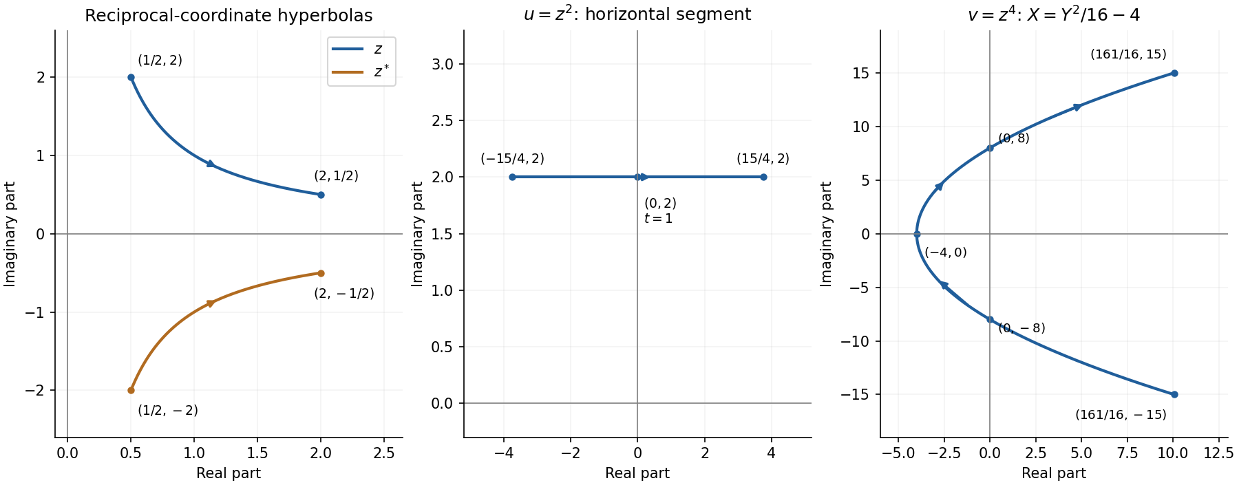
Trajectories under complex conjugation, squaring and fourth powers, with endpoints and axis crossings
. Details. Squaring givesThus is constant, while . The trajectory is the horizontal line segmentIt crosses the imaginary axis at , when , and never crosses the real axis. The middle panel shows the rightward direction.
Put . Part (b)(ii) gives , soThe parameter increases strictly from to . Therefore the imaginary part increases from to , while the real part is . The endpoints areThe real axis crossing is at , giving at . The two imaginary axis crossings satisfy , givingIn order, the trajectory passes from its lower endpoint through , then the leftmost point , then , to its upper endpoint. It is a right-opening parabola segment, traversed continuously upward as shown in the right panel.
From and , elimination of givesThis makes the real part a quadratic function of the imaginary part. There is no sign ambiguity because determines uniquely. The calculation illustrates power maps of a reciprocal-coordinate hyperbola.
In spherical coordinates, with polar angle and azimuth , the volume element isThe mass density is radial, so integrating over both angles givesWriting , this becomesAlthough the mass density diverges like near the origin, multiplication by the spherical volume element gives an integrable expression. Thus the central singularity does not produce infinite mass.
For , expand the exponential function in powers of :The constant and linear terms cancel in , givingFor , is exponentially small:The small- correction is smaller than every positive power of beyond the displayed linear term. In dimensional terms, the large- leading mass is , while the small- limit is .
The positive-domain graph starts with limiting value and limiting slope , then decreases towards the horizontal asymptote , with for large . In fact direct differentiation givesThe first inequality follows from for . Thus the graph is strictly decreasing and convex upward, with and no stationary points. The integral representation also shows its positivity.
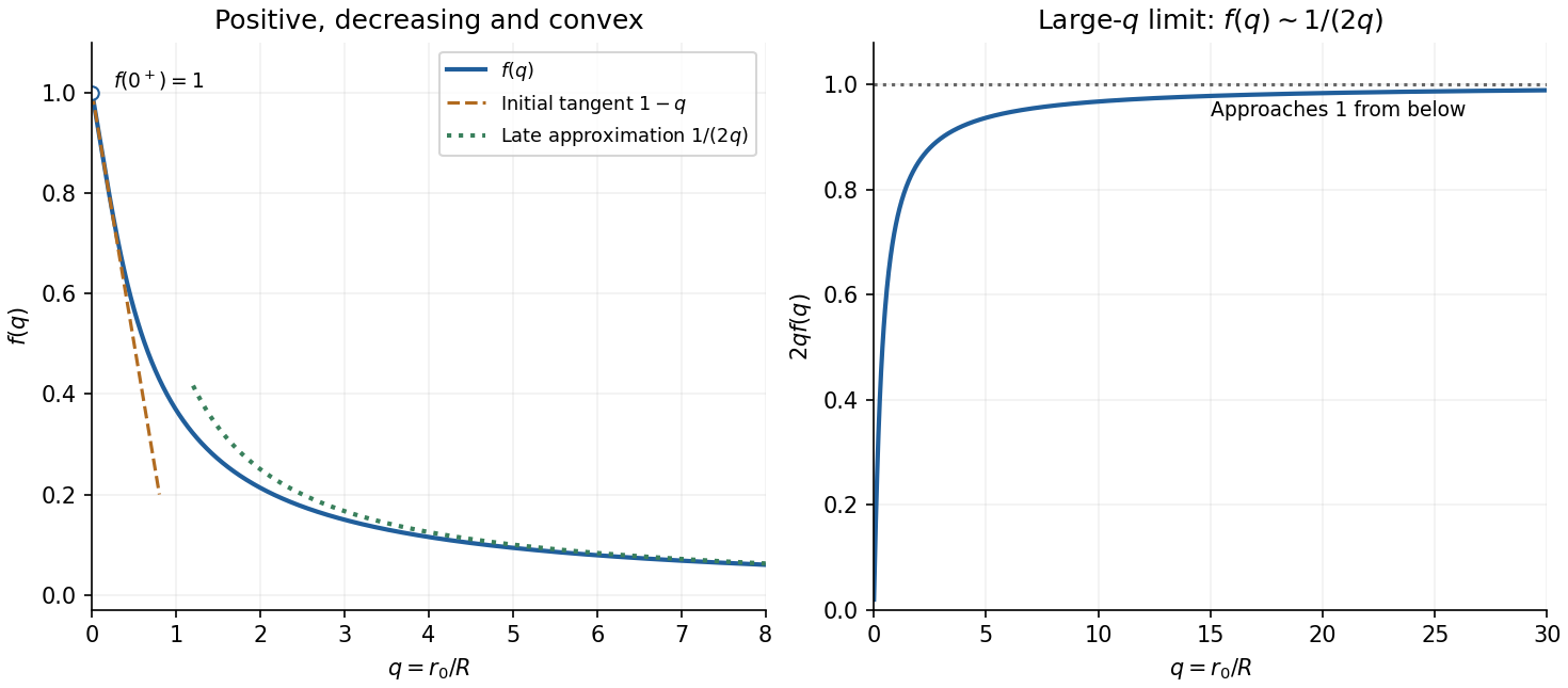
These properties belong to the reusable exponential spherical mass factor.
Use cylindrical coordinates , . The Jacobian determinant givesThe inequalities imply and . Thus the volume isEquivalently, integrating vertically first gives . The region is bounded by an elliptic paraboloid and its top disc; its volume is half that of the cylinder with base radius and height . Including or excluding the boundary surfaces does not change the volume.
The homogeneous linear differential equation is . Its characteristic equation is , with roots . The general real complementary function is thereforeThe two trigonometric solutions are linearly independent, supplying the two arbitrary constants required for this second-order linear ordinary differential equation.
Use the method of undetermined coefficients, choosing a particular solution . Substitution givesMatching the constant and cosine coefficients to gives , . ThusNeither forcing term is resonant with the homogeneous angular frequency one.
Combine the complementary function and particular solution:The boundary condition at zero gives , while that at gives . HenceThe two boundary conditions determine both constants uniquely; substitution at each endpoint gives zero.
First retain the equilibrium solution . Any nonzero real solution has constant sign on its interval of existence, since the polynomial right-hand side is locally Lipschitz and Picard-Lindelöf theorem prevents crossing the zero solution.
For a nonzero solution, the Bernoulli differential equation substitution givesThis linear ordinary differential equation has solution . Therefore every nonzero real solution isEither sign may be chosen and remains fixed. The restriction ensures ; nonpositive gives no nonzero real solution. These are maximal real intervals, and their restrictions are also solutions. As the right endpoint is approached, diverges in finite-time blowup. The substitution would have lost if it had not been checked separately.
For the force magnitude in Newton's law of universal gravitation, the total differential isDividing by the positive value gives the particularly useful relative formFor finite small changes this gives the first-order approximation to the fractional change; higher-order products of increments are omitted.
Set in the relative total differential and use the two equal mass increases:Thus the separation must increase by . In this special case the result is also exact: the mass product increases by , and preserving the inverse-square force requires , hence .
The original PDF specifies evaluation at ; the local TeX incorrectly gives . Write the scalar field explicitly as . Its gradient isA directional derivative measures rate per unit distance, so normalize the direction to the unit vector . ThenUsing the unnormalized direction vector would instead differentiate with respect to a path parameter, not distance, and would give a different scale.
The polar-coordinate Jacobian matrix and its Jacobian determinant areFor , the corresponding area element is . The determinant vanishes at , where the polar angle does not give a unique coordinate representation.
Put and . Logarithmic differentiation of the positive Gaussian function givesDifferentiating once more in space givesMultiplying by provesThe assumption ensures both the normalization and exponential denominator are defined. This is the heat kernel, with diffusion coefficient and centre .
For sufficiently differentiable on the interval between and , Taylor's theorem with its first terms readswhere lies between and . This is the Taylor theorem with Lagrange remainder. For example, on that interval gives . The finite formula does not assume that an infinite Taylor series converges to the function; that further conclusion requires the remainders to tend to zero.
The Maclaurin series of the hyperbolic cosine and cosine areBoth are even, so write their quotient as . Multiplication by the denominator gives coefficients and . Matching the numerator yields and . ThusThe denominator is nonzero near the expansion point, so division of the power series is valid there.
For , the definition of hyperbolic cosine simplifies the composite function exactly:Let . The geometric series givesAdding and dividing by two gives the requested Taylor expansion:The underlying infinite geometric expansion has .
Put . The local logarithmic series givesFor the infinite Taylor series, it is necessary to distinguish the real domain of the logarithm, , from its convergence interval about zero. Write . The complex zeros of are for integers , so the nearest logarithmic singularity to zero is at . The radius of convergence is therefore , giving convergence for and divergence for .
The two endpoints need separate checking. Factor off the nearest singularity:The quotient has a nonzero removable value at ; its other zeros are at with . Consequently it has a holomorphic logarithm on a zero-free disk larger than , which is a simply connected domain, and the Taylor series of converges absolutely at both real endpoints. At , the remaining series converges by the alternating series test. At , it is and diverges. Thus the full real convergence set isConvergence is absolute in the open interval and conditional at the left endpoint, where the sum equals . This endpoint distinction is an instance of isolating a logarithmic singularity to test a power-series endpoint.
Assume the three standard dice are fair and independent. For one die , a discrete uniform distribution on givesThe variance is . For the sum , linearity of expectation and addition of variances for independent random variables give
The sample space has equally likely ordered outcomes. The repeated value can be any of the six faces, giving six outcomes . Therefore
Choose the first face in six ways, the second in five ways avoiding the first, and the third in four ways avoiding both. ThusEach ordered outcome is equally likely in this sample space, so dividing the count by gives the probability.
To find the probability of exactly one pair, choose its repeated face in six ways, the distinct face in five ways, and which of the three dice has that distinct face in three ways. HenceAs a check, the disjoint events exhaust the sample space, and .
The sample space outcomes with qualifying sums have totals three, four and five. Their ordered patterns are , the three permutations of , and the three permutations each of and . Thus there are qualifying outcomes:
Of the ten outcomes in , all except have exactly one repeated pair. Hence . Applying Bayes' theorem in the requested direction,Equivalently there are nine favorable outcomes among the ninety outcomes in . This direct count confirms the conditional probability calculation.
The fundamental theorem of calculus, using continuity of near , givesThe lower endpoint is constant, so it contributes no additional term.
On the negative half-line, differentiation gives . The integration path from to stays away from the singularity at zero. ThereforeThis choice satisfies .
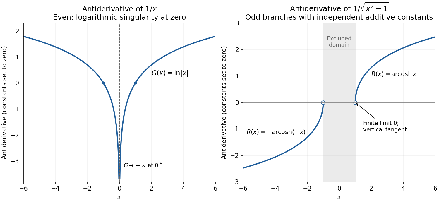
A suitable real antiderivative on the disconnected domain isFor , directly; for , and the chain rule again gives . The graph is even, crosses zero at , tends to on either side of zero, and tends to as . Independent additive constants may be chosen on the two disconnected half-lines; both are set to zero here.


Articles were limited to the first 100 out of 142 total.
Articles by others on the same topic
There are currently no matching articles.