Compare the total differential with and . The orthonormality of the coordinate basis gives the gradient in orthogonal coordinates:To obtain the curl without neglecting the variation of the basis vectors, write . The curl of a gradient vanishes, and the product rule givesLikewise because the system is right-handed. This cross product has zero divergence: . The divergence product rule applied to now givesCyclic permutation and linearity give the general component formulas described by divergence and curl from orthogonal coordinate gradients:andIn cylindrical coordinates, . The specified field has no dependence or component, soIt is an irrotational vector field for every exactly when . This statement is local to an angular coordinate chart: the component proportional to is not single-valued under .
With constant positive thermal diffusivity , no internal heat source and one spatial coordinate, the heat equation isSeparation of variables makes each spatial mode decay by . The endpoint conditions determine whether the initial triangular profile is expanded in a Fourier sine series or a Fourier cosine series.
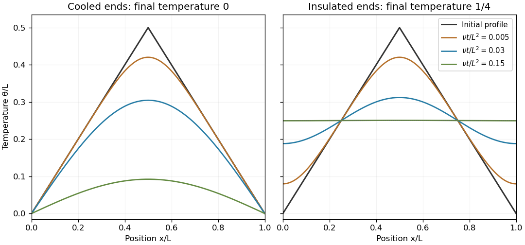
The same triangular initial temperature with cooled and insulated ends
. Original heat-equation solutions for several dimensionless times. Fixed zero-temperature ends cool the bar to zero; insulated ends preserve its initial mean and approach a uniform temperature. Details.
The cooled endpoints impose Dirichlet boundary conditions . The spatial modes are . Integrating the initial profile on its two straight segments givesThe heat flow from a triangular initial temperature with height is thereforeEvery nonzero mode decays, so as . There is no nonzero constant mode compatible with these endpoint temperatures.
By Fourier's law, insulation means zero outward heat flux. The Neumann boundary conditions are . The constant mode equals the initial integral average . For , the cosine coefficients areOdd modes and modes divisible by four vanish; write the remaining indices as . The heat flow from a triangular initial temperature with insulated endpoints givesThe nonconstant modes decay, so uniformly as . Integrating the heat equation gives , explaining the conserved mean. The cooled case tends instead to zero because heat leaves through its ends.
The initial triangle has nonzero endpoint slopes, so it is not compatible with the insulated condition at the corner . The series nevertheless recovers the continuous initial temperature and satisfies the insulated condition for every ; one should not assert continuity of its spatial derivative at that initial corner.
Use the Fourier transform conventionThese hold directly under suitable integrability and inversion hypotheses, and extend to square-integrable functions through the Plancherel theorem. At a jump, ordinary Fourier inversion uses the mean of the one-sided limits under the usual piecewise smooth hypotheses.
For the two-sided exponential, split the integral at zero:For the interval indicator, the Fourier transform of an interval indicator givesAt , the continuous limiting value is , the length of the interval. Changing the values at its two endpoints has no effect on the transform.
The convolution is . In this transform convention, the convolution theorem says , and Parseval's identity saysTo match the integral's scale exactly, set and . Then and , using the value one at zero. Their convolution is the box smoothing of a two-sided exponential with both scales equal to one:Its transform is precisely . Since is even, Parseval's identity reduces the requested integral toUse , and . Simplifying givesThe apparent singularity at is removable, and the integrand decays as , so the integral converges.
A Hermitian matrix obeys , where the dagger is conjugate transpose. If with , then . This scalar is real because its complex conjugate equals . Since , the eigenvalue is real.
For the Gram matrix, conjugate symmetry of the inner product givesThus is Hermitian. The assumption that the vectors form a basis additionally makes positive definite, though only Hermiticity is needed here.
For the general independence of eigenvectors for distinct eigenvalues, use induction. In a relation , applying gives . Independence of the first vectors makes each coefficient vanish. Distinctness of the eigenvalues then gives , and the original relation gives . No Hermitian assumption is required.
A real orthogonal matrix satisfies ; a complex unitary matrix satisfies . Their columns are orthonormal in the corresponding real or complex inner product.
Adopt the convention that a complex inner product is linear in its second argument, conjugate symmetric, and positive definite: , with equality exactly when . Conjugate symmetry and second-argument linearity then imply antilinearity in the first:For the specified real symmetric matrix use . Its upper block is the outer product , so it has one zero eigenvalue and one eigenvalue . A complete orthonormal eigenbasis isIf , the last two eigenvalues coincide and their eigenspace is the span of ; every nonzero vector in that span is an eigenvector. Since , the zero eigenspace remains one-dimensional.
An ordinary point of the normalized second-order equation is a point where both coefficient functions and are analytic in a neighborhood. Ordinary continuity is enough for a local existence theorem, but analyticity is the condition used for a convergent local power series solution.
A regular singular point is a nonordinary point for which and extend analytically across . These pole restrictions permit the Frobenius method.
The Wronskian is . If constants obey , differentiating gives . At any point where , these form an invertible two-by-two system, forcing . Thus the two solutions are linearly independent.
For the given equation, the normalized coefficients are and , so zero is a regular singular point. Substitute a Frobenius series , . The lowest power gives the indicial equationThe coefficient of givesFor either root the common factor is nonzero for , soWith leading coefficient one, the two independent solutions areTheir analytic series factors both have infinite radius of convergence, because the ratio of consecutive terms tends to zero for every fixed . The factor still gives the second solution a branch point at zero; it is not an entire function or an ordinary Taylor series there. On , the general real solution is . This is the , case of the exponential reduction of a confluent hypergeometric equation with equal parameters.
For the given weighted inner product, a self-adjoint operator obeys , including equality of its domain with the adjoint domain. In the differential-equation calculation this requiresfor all functions in a specified common domain, with endpoint conditions that remove the boundary form. Equality of these inner products by itself describes symmetry; the domain conditions complete the self-adjoint realization.
Divide the equation by to obtain its Sturm-Liouville form:Thus , and . For , the Lagrange identity for a Sturm-Liouville operator gives the endpoint form . A natural self-adjoint choice isUnder , these become the ordinary zero-derivative conditions at for . They therefore define the realization whose Neumann eigenfunctions of the Chebyshev differential operator are , with .
Boundedness alone does not choose these endpoint conditions: is also bounded but generally has a nonzero endpoint value of . Requiring bounded is a sufficient stronger regularity condition for the displayed zero-flux limits. Other self-adjoint endpoint choices are possible; the boundary form and the operator domain must specify which is intended.
Use the drift-removing substitution for a Dirichlet Sturm-Liouville problem, . It gives with . Positive requires ; zero or negative yields only the trivial solution under both endpoint conditions. HenceMultiplication of the original equation by gives . Thus the appropriate weighted inner product has weight , andMultiplying each eigenfunction by gives weighted norm one.
The homogeneous Cauchy-Euler equation has powers with . Boundedness at zero selects , and boundedness at infinity selects . Put for and for . Continuity gives . Since the operator is , the required delta-function normalization is . Thus , giving the bounded Green kernel for a radial Euler operator:In the requested notation, . The two expressions agree at .
With ordinary measure , the solution isFor bounded forcing these integrals converge and give a bounded solution. It is unique because no nonzero combination of is bounded at both ends. For a more general forcing, convergence and boundedness of the displayed integral must be checked.
The Green's function is nonpositive, so gives . If also , thenThe integral solution therefore givesBoth bounds are attained, by the constant forcings and , respectively. In particular, boundedness of the solution does not require it to approach zero.
Differentiate the integral formula using the Leibniz integral rule. Its two moving-endpoint terms cancel, leavingEach term before subtraction lies between zero and . ThereforeThe bounds are sharp at any fixed positive : put below that point and zero above it for the upper bound, or reverse those choices for the lower bound. If continuity of the forcing is required, smooth approximations approach the same bounds.
If the integrand has no explicit dependence, differentiate along a stationary path:The last equality uses and the Euler-Lagrange equation. This proves the Beltrami identity, the first integral .
If has no explicit dependence, the Euler-Lagrange equation becomes . ThusThe variable is then a cyclic coordinate. This is the case used for the azimuth in the ramp calculation.
For variations with , integration by parts gives . The fundamental lemma of the calculus of variations therefore gives the Euler-Lagrange equationFor the ramp, use conservation of energy from rest at the rim. The vertical drop is , so . The spherical surface arc length is . On a monotone segment described by , the travel time is consequentlyFor increasing this has the printed limits to ; for a descent, reverse the decreasing angular limits to keep time positive. The azimuth is a cyclic coordinate of this integrand. Its conserved derivative gives the first integral for the brachistochrone on a hemispherical ramp:Solving for its square yieldsFor a regular stationary path with finite , this tends to zero as the rim is approached. The ratio of azimuthal to meridional displacements is , which also tends to zero. Hence the initial direction is along a meridian toward the bottom. This conclusion concerns the initial heading; the later route can turn before reaching the bottom when its rim endpoints require a nonzero azimuthal displacement.
For example, impose homogeneous Dirichlet boundary conditions , and use variations vanishing there. Homogeneous Neumann boundary conditions are another choice removing the boundary terms. Put , , and . At a stationary function let . The quotient rule gives . After integration by parts, stationarity under every allowed variation givesso the fundamental lemma of the calculus of variations yields the stated Sturm-Liouville problem. Conversely an eigenfunction with those boundary conditions has and makes the quotient stationary. The lowest eigenvalue minimizes the Rayleigh quotient under the usual self-adjoint, lower-bounded hypotheses; higher eigenvalues are stationary values with orthogonality constraints when minimizing successively.
The hydrogen equation becomes . Its radial energy quotient is thereforeRegularity at zero and decay at infinity remove the boundary term . The condition fixes an arbitrary amplitude for these trial functions; it is not their three-dimensional probability normalization, which cancels from the quotient.
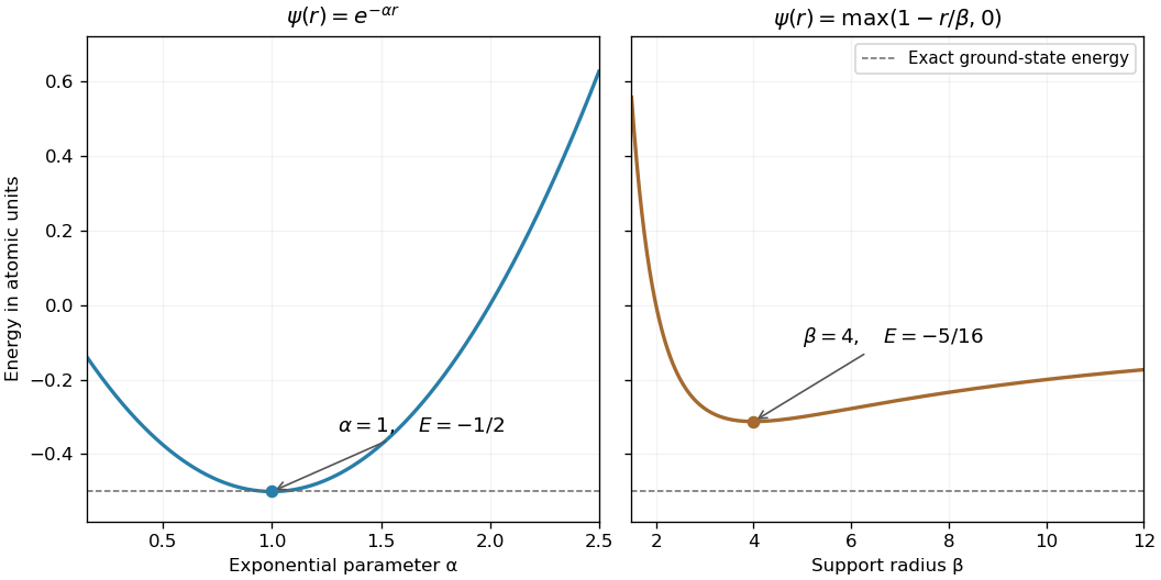
For , elementary exponential integrals give , , and . HenceFor the compactly supported linear trial for hydrogen, the norm, gradient and Coulomb integrals are , , and , respectively. ThusThe derivative changes from negative to positive at four, so this is the minimum over positive . The quantum variational principle gives upper bounds on the ground-state energy; the exponential trial is better, and in fact satisfies the exact differential equation at . It is the nodeless hydrogen ground state in the given units. The linear trial is admissible for the energy quadratic form despite its derivative jump at ; it need not possess a classical second derivative at that point.

For a separated harmonic function in polar coordinates, single-valuedness forces integer angular frequencies. The radial factors for frequency are , while frequency zero has a constant and . Finiteness at the origin excludes and .
The source's angular factor is in every term, as printed, rather than . The power-law angular mode for the planar Poisson equation givesHence, assuming the series permits termwise differentiation, the general finite, single-valued solution isThe arbitrary harmonic series must itself converge to a finite function on the prescribed disk. If , the source has a direction-dependent limit at the origin; the displayed potential still extends finitely there, but the equation at that point is understood weakly rather than as a smooth classical source.
For the special source, a particular potential is . Its boundary cosine term is canceled by , and the boundary sine term is supplied by . The resulting Dirichlet boundary conditions has solutionIt is finite at zero, has the required boundary values, and its Laplacian is .
The far radial derivative selects the growing frequency-one term . The matching decaying harmonic is . The no-penetration condition gives at , so . Thus the potential flow around a circular cylinder isThe remaining single-valued exterior harmonics are excluded by the zero radial derivative at the cylinder and the prescribed derivative at infinity, apart from the arbitrary additive constant. In particular the logarithmic radial term would have a nonzero radial derivative on the cylinder. A circulation term proportional to is excluded by single-valuedness of the potential.
Use Green's second identity in the source coordinate:Take and , the fundamental solution of the Laplace equation satisfying . With localized charge and the decaying potential, the boundary integral tends to zero on expanding spheres. The volume identity then gives , hence the Coulomb potentialConvergence of this integral and a condition fixing the potential at infinity are needed: mere pointwise decay of is not enough, and a harmonic function could otherwise be added. A bounded, compactly supported charge distribution is a sufficient setting for this derivation.
For the disk put . On its axis, every ring of radius is at distance , soFor subtract ; for add . This is the electrostatic potential of a uniformly charged disk with zero potential at infinity. The absolute value is essential for reflection symmetry and the correct behavior on the lower axis.
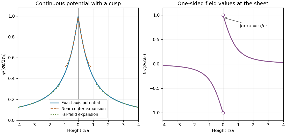

Write . The Taylor expansion gives the near-axis resultTo extend off the axis, work separately above and below the charged plane. In either source-free half-space the regular axisymmetric solid harmonics are . Matching the positive-axis coefficients, using , and then reflecting in the disk givesHere is a Legendre polynomial. The quadratic term is . The linear term is above and below; it represents the discontinuity of the normal electric field. A single regular spherical expansion across the entire charged sheet would incorrectly remove that jump.
For large , expand in to obtainThe axisymmetric exterior multipole expansion replaces each on the positive axis by . Reflection symmetry eliminates the odd multipoles, soThe leading term is the potential of total charge concentrated at the center; the next is its electric quadrupole correction. On either axis , recovering the same even axis potential.
For a complex derivative to exist, the difference quotient must agree along real and imaginary increments. These give and , respectively. Equating their real and imaginary parts gives the Cauchy-Riemann equationsFor , the components are and . The first equation requires , so ; the second requires , so . Thus zero is the only possible differentiability point. Directly,so . The function is differentiable at that isolated point but is not holomorphic on any neighborhood of it.
Use the chain rule with , . Then and . Substituting the Cartesian Cauchy-Riemann equations gives . Similarly . Thus, for , the polar equations areThe restriction is needed because the polar chart degenerates at the origin.
On the unit circle use with . The specified branch has there and . ThereforeThis is the circle integral of a logarithm with a radial branch cut, using the one-sided values at the cut crossing. The logarithm is discontinuous at that crossing, so the Cauchy integral theorem for a function holomorphic around a closed contour does not apply.
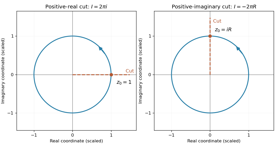

Choose the argument interval , which makes the logarithm real on the positive real axis and puts its cut on the positive imaginary axis. Parametrize . The constant term contributes , leavingEquivalently the cut-crossing point is , so the circle integral of a logarithm with a radial branch cut is . The different cut changes where the discontinuity lies on the circle; it is not merely an additive constant change of branch along the entire contour.
The residue theorem states that a positively oriented simple closed contour enclosing isolated poles and none on the contour has integral times the sum of their residues, provided the function is holomorphic elsewhere inside. Near a simple zero of , . HenceFor , this gives for every integer .
To evaluate the real integral, integrate around an upper semicircle, with a small upper semicircular indentation excluding zero. Use the branch real on the positive axis and with argument between zero and in the upper half-plane. The large arc tends to zero as and the small arc as . The only enclosed pole is , whose contribution isOn the negative real axis the upper boundary value is . The two real segments therefore contributeComparing real parts yieldsThe integral is absolutely convergent at both zero and infinity, so no principal-value interpretation is needed.
For causal functions the convolution is . In a half-plane of absolute convergence, changing variables in its Laplace transform and using Fubini's theorem givesThis proves the convolution theorem for Laplace transforms. Transforming the differential equation gives . The direct transform pairs and then giveFor a continuous forcing, call the last term . The Leibniz integral rule gives and . Also . Thus both the original equation and the initial values hold.
For an impulse at positive time , the Dirac delta evaluates the convolution, yieldingHere is the Heaviside step function. The displacement remains continuous at , while its derivative jumps upward by one, exactly as required by integrating the differential equation across the unit impulse.
An isotropic tensor has unchanged components under every rotation of the Cartesian axes. Under proper rotations in three dimensions, rank one has no nonzero isotropic tensor, rank two has , and rank three has . Here is the Kronecker delta and the Levi-Civita symbol. If invariance under reflections is also required for a true tensor, the rank-three case vanishes; is then a pseudotensor.
The velocity gradient tensor for the given field isIts symmetric part, the strain-rate tensor if is interpreted as a velocity, isThe antisymmetric part has the specified ordering , withThe index ordering matters for this sign; it agrees with a local rotation velocity . This is the axial part of the scalar, symmetric-traceless and axial tensor decomposition, retaining the trace inside the symmetric part here.
At the specified point, . The upper block has characteristic polynomial . Thus the principal values and unit eigenvectors areThese mutually orthogonal directions are the principal strain rates' axes for this local field; reversing an eigenvector does not change its axis.
A normal mode has all coordinates following one fixed displacement pattern with a common time factor. Its normal frequency is that factor's oscillation frequency; normal mode coordinates are amplitudes in a basis of such patterns, making the linear equations independent. A zero-frequency mode can instead have constant velocity along a symmetry direction.
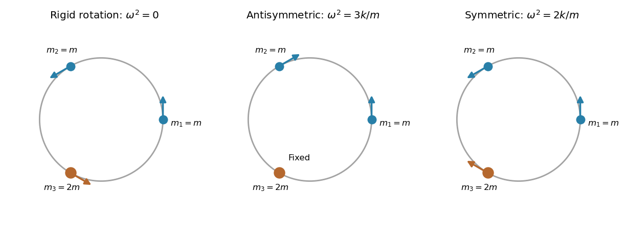
For the unit circle, each angular displacement equals its corresponding arc displacement. The kinetic energy and change in potential energy areAny common spring prestress changes only the constant , because the sum of the three arc lengths is fixed. The Euler-Lagrange equations giveThese are the normal modes of three beads connected by springs on a circular hoop, with third mass . For , their three mode vectors and squared angular frequencies areThe zero mode rotates the entire configuration without stretching a spring. The antisymmetric mode moves the equal masses oppositely while leaving the third fixed. In the symmetric mode the equal masses move together against the third, with zero total angular momentum. These vectors are orthogonal in the mass inner product with matrix .
Writing gives independent equations , , . In particular , retaining possible slow common rotation. For , the two positive frequencies coincide at ; their two-dimensional space is all patterns with .

A right coset of in is . Right multiplication by is a bijection , with inverse , so every right coset has elements. The analogous map proves the same assertion for left cosets.
Write the displayed matrices as . Direct multiplication givesAll new coordinates are integers, so the set is closed. Matrix multiplication is associative, the identity is , andwhich also has integer coordinates. Thus it is the Integer Heisenberg group.
The subset contains the identity, and multiplication and inversion add or negate , so it is a subgroup. Its right cosets areThey are exactly the sets with fixed integer coordinates , as described by cosets of a coordinate subgroup of the integer Heisenberg group. The factor order is essential; multiplying by on the other side would also change the upper-right coordinate by .
Let be a quarter-turn and a reflection of the square. The dihedral group is generated by with and , and its elements are . Two generators are minimal because this group is not cyclic. Its subgroups of order two are and for . Its subgroups of order four are , and .
A group homomorphism obeys for all elements; a group isomorphism is a bijective group homomorphism. Take the rotation subgroup and defineThe quaternion element has order four, so the map is well defined modulo four, preserves products and is injective onto . Surjectivity onto all eight quaternion elements is not required of a homomorphism.
A cyclic group is generated by the powers of one element. The final claim needs the usual qualification no nontrivial proper subgroup, and : the trivial subgroup is proper in every nontrivial group, even one of prime order. With that interpretation, if has prime order , Lagrange's theorem permits only subgroup orders one and . Conversely, if its order is composite, choose a divisor with . The subgroup has order , strictly between one and . This proves the assertion described by groups with no proper nontrivial subgroups.
A group representation is a homomorphism into invertible linear maps. It is a faithful representation when it is injective, equivalently when its kernel contains only the identity. A faithful real two-dimensional representation of the cyclic group of order four isThese are rotations of the plane through . Since and , their multiplication agrees with the group, and all four matrices are distinct.
For any invertible , set . Thenso this also is a group representation. The character of a representation is . For the displayed quarter-turn representation, its values on are .
The trace is invariant under a similarity transformation, by cyclicity of the trace:Hence equivalent representations have the same character of a representation.
If , the representation law gives . Trace invariance under this similarity transformation givesThus the character of a representation is constant on every conjugacy class.
Articles by others on the same topic
There are currently no matching articles.