Using Cartesian coordinates, the Levi-Civita symbol and the Einstein summation convention, the constant-vector assumption givesRecognizing the divergence and directional derivative provesHere the contractions use the Kronecker delta.
For an oriented piecewise smooth surface with boundary , Stokes theorem stateswhere the orientations obey the right-hand rule and is continuously differentiable near . Apply it to . The scalar triple product givesThe last integrand is , as the component formulashows. Since is arbitrary, the cross-product form of Stokes theorem follows:The derivatives in the surface expression act on , not on the surface element.
For the specified square, the path is clockwise when viewed from positive , so the compatible unit normal is . On the first and fourth edges, and are parallel, giving zero cross product. On the second edge, and runs from to , so contributes . On the third edge, and runs from to , so the contribution is . Thus the line integral is .
For an independent surface integral, and for the position vector field. Its integrand is therefore . The square has unit area and downward orientation, giving
For a spherically symmetric number density, the radial Laplacian is . Applying separation of variables and choosing the separation constant givesso the ordinary differential equations areThe radial problem is an eigenvalue problem for with Dirichlet boundary conditions, hence : multiplying the radial equation by and integrating gives for a nonzero regular mode vanishing at .
To solve it explicitly, set , corresponding to the suggested power . The equation reduces to , soFiniteness at the origin forces , and the Dirichlet boundary condition at requires for an integer . The absence of interior zeros excludes , selecting the fundamental normal mode. If denotes the initial central density, the result iswhere the sine ratio is defined as at the origin. It is strictly positive in the interior for every finite time. The arbitrary positive scale cannot be fixed without additional initial data.
The spatial factor is time independent, so the density and the total neutron population have the same exponential growth rate. Thus the spherical reaction-diffusion growth threshold isAt equality the fundamental mode is stationary; below it the mode decays. For fixed , the equivalent critical-radius condition is . This is the competition between multiplication in the bulk and diffusion loss at the surface in the stated dimensionless model.
The homogeneous equation is a Cauchy-Euler equation. Trying gives the repeated indicial rootHence, for ,Both independent solutions diverge at the origin, so no nonzero homogeneous combination satisfies the zero-origin conditions by continuous extension.
For a source point , finiteness on forces the Green function to vanish on that side. On , continuity and the unit first-derivative jump requireUsing the homogeneous solutions gives the causal Green function for a repeated-root Euler operatorIndeed, the Wronskian of and is , and direct differentiation gives . Since is continuous, its second derivative produces precisely a unit Dirac delta, with no derivative of a delta. For each positive source it is identically zero near the origin, so both required origin values vanish. The differential operator itself is interpreted on ; no value of its singular coefficients at zero is needed.
Integrating against the forcing yieldsThe last integral equals , by integration by parts or differentiating . ConsequentlySubstitution gives , while . The divergent homogeneous solutions prove uniqueness in the regular class. No boundary condition at infinity was imposed or required.
Complete the square in the Fourier transform exponent:The supplied shifted Gaussian integral therefore givesThis is the Fourier transform of a Gaussian, with angular-wavenumber convention .
Take the spatial Fourier transform of the heat equation. Two integrations by parts, with decaying fields and first derivatives at infinity, give . Thus each mode satisfies the ordinary differential equationInserting the transformed initial condition and integrating the time equation givesFinally set . The inverse Fourier transform, evaluated by the same Gaussian identity, givesEquivalently the Gaussian initial data for the heat equation evolve asThe profile broadens and its peak decreases, while its total integral remains , as required by diffusion without loss on the whole line. Direct differentiation verifies the equation and the initial limit.
Let be the linearly independent eigenvectors, and form . This matrix is invertible and , where . Hencewhich proves diagonalizability.
If , then are linearly independent eigenvectors of with the same eigenvalues. Explicitly, with ,Thus matrix similarity preserves diagonalizability.
The spectral theorem for a Hermitian matrix supplies a unitary matrix and real diagonal matrix with . This single representation gives all three conclusions below.
For a positive integer , cancellation of gives . The trace is invariant under matrix similarity, since , and the determinant is multiplicative. ThereforeThis includes zero eigenvalues without requiring to be invertible.
The convergent power series defining the matrix exponential gives , with . Hence the matrix exponential determinant identity isThe diagonalization proof uses the given Hermitian hypothesis; the identity itself holds for every square real or complex matrix.
Applying to an eigenvector gives , so each eigenvalue is either zero or one. If all are one, the spectral theorem gives , hence and . Otherwise, if eigenvalues are one, with , thenThus the trace of this orthogonal projection equals its rank, including for the zero matrix.
The decomposition is . Both matrices are Hermitian: and , directly from their definitions and complex conjugation of . The matrix is the Hermitian part of a matrix, whereas is the Hermitian matrix obtained by dividing the skew-Hermitian part by .
Multiply the eigenvalue equation on the left by . The unit vector normalization is , soNo normal matrix assumption on is needed: this is an identity for each normalized eigenvector.
For any Hermitian matrix , the scalar is real because its complex conjugate equals . Applying this to in part (a) givesThese are the real and imaginary quadratic forms associated with the numerical range of .
Use the inner product on . The distinct real eigenvalues permit a full orthonormal eigenvector expansion; the two child solutions establish that expansion and apply it to the proposed quadratic form.
For , Hermitian symmetry givesDistinct eigenvalues therefore imply for . Together with the unit normalizations,The mutually orthogonal nonzero vectors are linearly independent and span the -dimensional space, so they form an orthonormal basis. Here is the Kronecker delta.
Expand , where . By orthonormality,Since the spectrum avoids , each is either below or above , making every product strictly positive. This proves positivity of a quadratic polynomial across a spectral gap:In particular for every nonzero . For , ; the printed strict claim for an arbitrary vector must exclude this case.
The complex potential of a two-dimensional potential flow combines the velocity potential with the stream function . For its holomorphic representation, the Cauchy-Riemann equations are and .
Since , its divergence is the Laplacian of the velocity potential. Using the Cauchy-Riemann equations and equality of mixed partial derivatives givesThus this is an incompressible flow, and is a harmonic function.
The derivative of a holomorphic function can be evaluated using an increment along the real axis:Identifying the components of the gradient gives
For , the defining Gamma integral converges at zero and at infinity and defines a holomorphic function. The Gamma function recurrence then supplies its meromorphic continuation to the rest of the complex plane, as used below.
For , integration by parts givesThe boundary term vanishes because at zero and exponential decay dominates any fixed power at infinity. ThusThis also gives for nonnegative integers, linking the Gamma function to the factorial.
Iterate the Gamma function recurrence to obtain, near for ,The numerator is holomorphic and equals at . Exactly one denominator factor, , vanishes; the product of the remaining factors there is . Thus there is a simple pole, with Gamma function residue at a nonpositive integerFor the empty product is one. The same recurrence with a sufficiently large shift defines the continuation at every point away from these integers, so no further poles occur. At the poles, the recurrence is an identity of meromorphic functions, rather than an equality of finite values.
Insert the power series and equate the coefficient of . In the Legendre differential equation this givesHence the recurrence relation isThe free coefficients generate the independent even and odd series, respectively. They converge at least for , up to the nearest singular points of the equation.
For a nonnegative integer , the chain of the same parity as reaches , where the numerator of the recurrence relation vanishes. The next coefficient and every later coefficient in that chain are zero, producing a polynomial of degree . Normalizing it at gives the Legendre polynomial .
The opposite-parity chain never reaches . Its other possible zero, , is negative and cannot occur, so a nonzero initial coefficient produces a nonterminating power series. It is linearly independent of and can be scaled to the Legendre function of the second kind .
The degree statement requires , as the examples in part (c) indicate. For a negative integer , the same equation has the nonnegative degree , because . A polynomial cannot literally have negative degree.
For the terminating even solution is constant; for the terminating odd solution is proportional to . For , the recurrence gives ; for it gives . Imposing the Legendre polynomial normalization at yields
Let . Differentiation cancels the cross terms, and the Legendre differential equation givesThus , sowith independent of on each interval avoiding the singular endpoints. This is the Abel identity. Linear independence forces , and its value depends on the chosen normalization of .
Since , part (d) gives . A partial fraction decomposition and integration give, for ,The condition at zero fixes . Thus the full conclusion from the stated condition isThat condition alone does not fix the multiplicative constant. With the usual Legendre function of the second kind normalization , one has . On real exterior intervals replace the logarithm by ; complex continuation requires a choice of logarithm branch.
Take endpoint-preserving variations , with . The first variation of the functional is ; integration by parts supplies the differential equation and its conserved quantity below.
The boundary term vanishes, so stationarity and the fundamental lemma of the calculus of variations give the Euler-Lagrange equation
If is independent of , then and the Euler-Lagrange equation reduces to . Therefore the first integral isThis is the conserved generalized momentum for a cyclic coordinate.
By Fermat principle, a light ray makes optical travel time stationary. Multiplication by the constant vacuum speed of light does not change the stationary paths, so the functional can be taken to be the refractive index integrated over arc length. The constant denoted below is an integration constant, not that vacuum speed.
The integrand has no explicit dependence on , so part (i) givesFor positive refractive index and a regular graph with , squaring and then restoring the sign of yieldsIt is the continuous-medium version of Snell's law, expressing conserved horizontal optical momentum. The Euler-Lagrange equation establishes stationarity; on a monotone-height segment, convexity of the integrand in also gives a minimum among graphs with fixed endpoints.
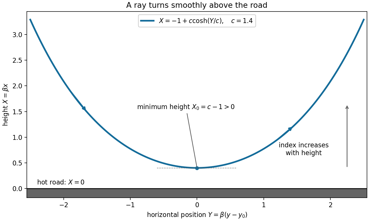
For the displayed form take and . Substitute in the first integral:Inverting the hyperbolic cosine gives the catenary light ray in a linear refractive indexThe minimum occurs at and , so the integration constant has the specified meaning. The integral above describes the graph branch; the other sign of the square root continues it smoothly to the other side of the turning point in .
The signed-constant qualification matters: for in part (a), integration reverses horizontal direction, and the positive prefactor in the full catenary is , with minimum height . The printed expression presupposes . The separate case gives constant, a vertical ray. At the turning point diverges, so is not a single regular graph across it, although is smooth.
For , the catenary has a positive minimum height above the road. Its derivatives areThus the light ray is symmetric about , descends towards a horizontal tangent at its minimum, and then rises. It never intersects the road. This smooth upward bending in the refractive index gradient produces an inferior mirage, without reflection at the road.

Write the energy form as and the weighted squared norm as . For real coefficients and appropriate homogeneous boundary conditions, the Sturm-Liouville problem is the stationary-point equation for their Rayleigh quotient .
One suitable choice is homogeneous Dirichlet boundary conditions, , with variations vanishing there. Assume real and the stated positive . Introduce a Lagrange multiplier for . For real variations, integration by parts givesThe boundary term vanishes, so the fundamental lemma of the calculus of variations yieldsMultiplying this equation by , integrating, and using the boundary conditions gives . Thus the multiplier, the eigenvalue, and the constrained stationary value coincide. Conversely every normalized eigenfunction makes the first variation vanish for all tangent variations satisfying .
Homogeneous Neumann boundary conditions, at both endpoints, or mixed Dirichlet and Neumann conditions also work with this energy form. General Robin boundary conditions require the corresponding boundary terms in the form; they cannot simply be inserted into the displayed unmodified integral.
For a regular self-adjoint problem with a lowest eigenvalue and a complete orthonormal eigenbasis in the weighted inner product, expand an admissible trial function as . ThenThe Rayleigh-Ritz variational principle therefore provides the upper boundChoose a family satisfying the essential boundary conditions and finite energy, evaluate the quotient, and minimize over its parameters. Enlarging the trial family can only improve or preserve the bound; equality is attained if it includes an exact ground eigenfunction. For a finite linear trial space, this becomes a generalized matrix eigenvalue problem.
Here and on the whole real line. The quantum harmonic oscillator energy form is . Admissible trials have a square-integrable weak derivative and finite potential energy; they need not have a classical second derivative everywhere.
Put , with . Direct integration confirms the normalization:The kinetic energy and potential energy terms in the dimensionless Rayleigh quotient areThus . Differentiating with respect to gives , so the unique minimizing width is . The two energy contributions are equal there, and the compact parabolic trial bound for the quantum harmonic oscillator isThe trial is continuous and zero at , so its weak first derivative is inside and zero outside. The jumps of that derivative do not add delta terms to the first derivative, and its squared norm is finite. The energy-form calculation is therefore valid even though the trial does not belong to the operator domain of the harmonic oscillator. Applying the second-derivative operator naively and omitting its endpoint distributions would be incorrect.
For any nonzero constant , differentiating gives . HenceIt is indeed the lowest eigenvalue, since the factorization makes , with equality for this Gaussian. The variational bound exceeds the exact value by , or about .
The PDF's prefactor does not normalize this wavefunction: its squared norm is . The normalized ground state has prefactor . This normalization error does not affect the eigenvalue, because the equation is homogeneous in the wavefunction.
For real positive weight , the weighted inner product isThe functions must have finite weighted norm; the conjugate is omitted for real functions. Multiplying the differential equation by givesThus the Sturm-Liouville form has , and . With the positive-sign spectral convention defineThe existing Laguerre differential operator on polynomials uses the opposite operator , with eigenvalues ; keeping this sign convention explicit avoids confusing the two descriptions.
For admissible , integration by parts givesThe boundary form must vanish for every pair in the self-adjoint domain. In the usual regular-at-zero Laguerre realization one imposes , excluding the logarithmic branch; at infinity one uses the weighted square-integrable domain with vanishing boundary form. A condition would be inappropriate for polynomial eigenfunctions. For any pair of polynomials, the factor makes the boundary form zero at zero, while the exponential beats all polynomial growth at infinity. These functions also have finite weighted norms.
Self-adjointness yields , giving orthogonality of Sturm-Liouville eigenfunctions:For the specified polynomials, direct differentiation gives and . Hence their eigenvalues in the displayed convention are 1 and 3, respectively, or −1 and −3 for .
To find the quadratic, put . The equation reduces to . Thus , . Since ,These are scalar multiples of the Laguerre polynomials of degrees one, three and two.
For , the first integral is , so all solutions with the prescribed interior normalization areTwo independent choices areThey both equal one at , and their Wronskian is . For sufficiently large , the last unit interval contributes at least , proving that . These are the zero-eigenvalue solutions of the Laguerre differential equation, with the second expressible through the exponential integral. It also has a logarithmic singularity at zero and is not an admissible polynomial or weighted square-integrable eigenfunction. An interior value alone does not enforce the endpoint conditions of the spectral problem.
If , write . The first condition gives , and the second gives . Together they force , so this case contributes only the zero solution.
If , write . The first condition gives . The second becomesA nonzero solution therefore requires , giving and time factor .
If , write . Now , and the remaining condition is . Thus , . Choosing a convenient amplitude gives . The complete Sturm-Liouville eigenfunction expansion is consequentlyThese are self-adjoint separated Robin boundary conditions: the boundary form vanishes because both functions satisfy at each end. The regular interval problem has a complete orthogonal eigenbasis; the calculation includes its one negative eigenvalue for , not only its positive ones.
To project the initial data, calculate the squared norms:The second identity uses the half-unit integrals of and and the zero integral of their product. By orthogonal projection,For square-integrable , the initial expansion is understood in that norm. Classical agreement of boundary derivatives at requires compatible smoother data.
This is Robin diffusion with a growing mode, in the reflected version of its positive-coordinate-derivative example. Growth is not a contradiction: the outward derivative is at the left endpoint, so these conditions are not dissipative outward-normal conditions at both ends. Indeedand the boundary can supply energy. The growing contribution is absent exactly when the displayed integral defining vanishes.
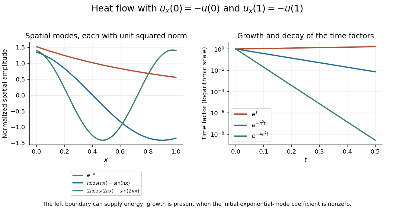
The growing exponential mode and two decaying oscillatory modes satisfy the same coordinate-derivative boundary conditions
. Details. 
The terms cancel in . For a ball , the product rule and divergence theorem give Green's second identity in the formThus the whole-space integral vanishes when this boundary term tends to zero. For example, uniform bounds and , with , make it .
Pointwise vanishing alone, as stated in the source, is insufficient. Smooth fields agreeing with and outside a ball both tend to zero, but their distant boundary integral is . One may smooth them inside the ball without changing that flux. The requested zero identity therefore needs sufficient decay or boundary/radiation conditions that actually eliminate the boundary term.
For the generalized plane wave eigenfunctions, their orthogonality is distributional:Here is the Fourier representation of the Dirac delta function. These eigenfunctions are not ordinary square-integrable functions or decaying test fields.
Expand and define . Since , projection of the source equation gives . Formally dividing and substituting back givesAt the shell , a pole prescription is required; homogeneous solutions can otherwise be added. The formula is an inverse of the Helmholtz equation with that convention still to be selected.
Let denote the kernel in this source formula, so . Put and align the Fourier polar axis with . Angular integration givesConsequently the radial Fourier representation of the Helmholtz Green function givesThe last Green function written in the PDF has the opposite denominator. It is obtained by setting , the common convention :Thus the two displayed source and Green formulas are consistent only when this minus sign is retained; cannot also be the positive-delta inverse kernel.
Finally the integral is not an ordinary improper integral across . A Cauchy principal value yields . The outgoing prescription yields the outgoing Green function for the three-dimensional Helmholtz equation, ; the opposite sign gives the incoming wave. The Sokhotski–Plemelj formula accounts for their difference. The source does not specify which prescription is intended, so the boxed radial expression must be read with one chosen consistently.
For a counterclockwise simple contour containing , and analytic on a neighbourhood of its interior and boundary, the Cauchy integral formula isFor the required rational integral, use partial fraction decomposition:Both points lie inside . Applying the formula with the constant analytic function one gives for each of the two terms. They cancel, soReversing the circle's orientation would leave this zero result unchanged.
On a positively oriented contour encircling once inside an annulus of analyticity, the Laurent series coefficients areThis follows by inserting the convergent Laurent expansion and integrating term by term: only the term with exponent has nonzero contour integral. Uniform convergence on compact circles in the annulus justifies that step.
For the function at hand,The geometric series converges for , and the pole at zero excludes the centre. ThusThe coefficients are for and zero for . The coefficient formula gives the same result on : , and expansion of selects exactly those coefficients.
The annulus is essential. For , expand instead in inverse powers:These are different Laurent expansions about the same centre on the two annuli separated by the singularity at . The series requested in the PDF is the inner one, not a global expansion.
For integrable , define their convolution by . Absolute integrability of the double integral permits Fubini's theorem. With ,The convolution theorem, together with uniqueness of the Fourier transform, therefore identifies the inverse transform of that product with . With the stated convention the inverse carries , so there is no extra factor in the convolution itself.
Now take . For , split the convolution at and :The convolution of two even functions is even, so the self-convolution of a bilateral exponential givesIn particular the centre value is one; both pieces extend continuously there.
Splitting the Fourier integral at zero givesHence . The Fourier inversion theorem yieldsThe integral is absolutely convergent. At it gives , providing a normalization check.
Articles were limited to the first 100 out of 112 total.
Articles by others on the same topic
There are currently no matching articles.