Past exam of the mathematics course of the year 2 of the natural sciences course of the University of Cambridge / 2013 / Paper 1

Using the Levi-Civita symbol and the Einstein summation convention in Cartesian coordinates, the product rule givesThe cyclic permutation in the first term preserves the sign, whereas exchanging the first two indices in the second reverses it. Recognizing the two curls proves

The divergence theorem states that a continuously differentiable vector field $\mathbf{F}$ on a volume $V$ with piecewise smooth closed boundary $S$ satisfieswhere $\hat{\mathbf{n}}$ is the outward unit normal. Take $\mathbf{F}=\nabla a\times \mathbf{B}$. Since the curl of a gradient is zero for a twice continuously differentiable scalar field, part (i) givesIntegrating this identity and applying the divergence theorem proves

Direct differentiation givesOn the unit disk $D$, polar coordinates give ${\int }_D{y}^{2}dA=\pi /4$, ${\int }_{D}xdA=0$ and ${\int }_{D}dA=\pi$. Consequently the volume integral isFor an independent surface integral calculation, the relevant cross product isThe bottom face contributes ${\int }_{D}xydA=0$ and the top contributes ${\int }_D(-h{y}^2-xy)dA=-\pi h/4$. On the cylindrical side, put $x=\cos \theta$, $y=\sin \theta$, $\hat{\mathbf{n}}=(x,y,0)$ and $dS=d\theta dz$. The flux density is $x^3+2xy{z}^2+2y^{2}z-x{y}^2$. All terms except $2y^{2}z$ integrate to zero because they are odd functions of $x$ or $y$, givingThus minus the total outward flux is $-(\pi h^2-\pi h/4)$, in agreement with the volume integral.

For separation of variables, take $u(x,t)=X(x)T(t)$ in the damped wave equation. Dividing by $c^{2}XT$, with $c>0$, gives $X^{\prime \prime }/X=(T^{\prime \prime }+\alpha T^{\prime })/(c^{2}T)=-k^2$. The separated ordinary differential equations are thereforeThe negative separation constant anticipates the positive spatial eigenvalues selected by the fixed endpoints.

An even function satisfying the spatial equation has $X=C\cos (kx)$. The Dirichlet boundary conditions require $\cos (kL)=0$, so the allowed wavenumbers areThere is no nonzero zero-wavenumber mode. With $T=e^{-\alpha t/2}S$, the time equation becomes $S^{\prime \prime }+{\omega }_n^{2}S=0$, where ${\omega }_n^2=c^2{k}_n^2-{\alpha }^2/4$. Thus superposition of the even normal modes givesThis uses completeness of the even Fourier series modes. Imaginary ${\omega }_n$ describe overdamping. At critical damping, ${\omega }_n=0$, the two displayed exponentials coincide: the complete time factor must instead be $e^{-\alpha t/2}(C_n+D_{n}t)$. This repeated-root exception is necessary for a genuinely general solution.

The angular frequency of an underdamped mode isFor ordinary damping, $\alpha \ge 0$, mode $n$ oscillates precisely when $\alpha <cn\pi /L$. In particular, all modes, including the fundamental, oscillate when $\alpha <c\pi /L$. There are some oscillatory modes for every finite $\alpha$, since the allowed $n$ are unbounded; no finite damping coefficient overdamps the entire ideal string spectrum.

If $\alpha <0$, the same mode has negative damping: oscillatory amplitudes grow as $e^{|\alpha |t/2}$. For modes with real characteristic roots, both roots are positive, since $|\alpha |/2>\sqrt{{\alpha }^2/4-c^2{k}_n^2}$. Hence those modes also grow. Negative damping makes the equilibrium unstable.

Let $d_n$ be the even Fourier coefficient of the initial displacement, with the normalization ${\int }_{-L}^L{\cos }^2(k_{n}x)dx=L$. Writing $s_n=\sin (n\pi /2)=(-1{)}^{(n-1)/2}$ givesZero initial velocity requires the real modal time factorOne consistent choice in the question's complex representation is thereforeFor real ${\omega }_n$, $B_n=\overline{A_n}$; the real-part notation otherwise makes the complex coefficients nonunique. For imaginary ${\omega }_n$, the same formula is interpreted using hyperbolic functions. Its limit at ${\omega }_n=0$ is $d_n{e}^{-\alpha t/2}(1+\alpha t/2)$.

For $l/L\to 0$ at fixed mode number,which can be substituted into $A_n,B_n$ above. The profile specified at $t=0$ is actually nonzero at $x=\pm L$. Thus for finite $l/L$ it cannot be the initial data of a solution continuous at the initial endpoint corners with fixed endpoints. The Fourier series reproduces it in the open interval, with zero endpoint values; it is an L2 space initial-data interpretation. The assumption $l\ll L$ makes this compatibility error exponentially small, rather than exactly zero.

The substitution $y=e^{x}g$ reduces the homogeneous linear differential equation toA first integration gives $g^{\prime }=Cx{e}^{-x}$, and a second gives $g=D-C(x+1)e^{-x}$. HenceThe Wronskian of $1+x,e^x$ is $x{e}^x$, so they are linearly independent on either side of zero. At zero the differential equation has a regular singular point. The displayed solutions extend analytically through it; their linear combinations describe the global solutions when two continuous derivatives are required there. If no matching condition is imposed, the two sides have independent constants.

Use the boundary-adapted homogeneous solutionsFor a source point $\xi \ne 0$, the Green function isIt vanishes at both endpoints and is continuous at $x=\xi$. Its first derivative has the jumpas required for a monic second-order differential operator with a Dirac delta source. Away from that source it is a homogeneous solution and extends smoothly through $x=0$.

The interior singular point requires a qualification. This is a Green kernel with a vanishing Wronskian at an interior singular point, with a $1/\xi$ singularity in its source variable. It is not an ordinary integral inverse for unrestricted forcing. For smooth forcing $f(\xi )=\xi q(\xi )$, however, the product $Gf$ extends continuously at zero and the integral is well defined. This includes part (iii). We use solutions with two continuous derivatives across zero, interpreting the equation there after multiplication by $x$. For such a solution, expansion at zero forces $f(0)=0$; arbitrary nonzero forcing at zero cannot satisfy this regularity. Merely imposing one continuous derivative would leave a piecewise homogeneous ambiguity, so the original singular coefficients alone do not specify an unrestricted boundary-value inverse.

The source factor cancels the singular denominator of the Green function. Splitting the integral at $\xi =x$ givesUsing $\int (1+\xi )e^{-\xi }d\xi =-(\xi +2)e^{-\xi }$, these two integrals are $e-(x+2)e^{-x}$ and $5/2-x-e(x+2)e^{-x}/2$, respectively. Simplification givesThe exponential and linear terms are homogeneous solutions, while direct differentiation gives $L(-x^2)=x$ for $x\ne 0$. Also $y(-1)=y(1)=0$, and the expression is analytic through zero. Uniqueness in this regular class follows because any difference is a global linear combination $A{e}^x+B(1+x)$: the left boundary forces $A=0$, and the right then forces $B=0$.

First take $f,g\in L^1(\mathbb{R})$, so Fubini's theorem applies to the cross-correlation double integral. With $s=x+y$, the Fourier transform isThe complex conjugation and the sign in $x+y$ are both essential to this convention.

Set $g=f$. The cross-correlation at zero is $h(0)={\int }_{\mathbb{R}}|f(x){|}^{2}dx$, while part (i) gives $\hat{h}=|\hat{f}{|}^2$. Evaluating the inverse Fourier transform at zero yields the Parseval identityThis derivation is immediate for Schwartz functions, for which all integrations and Fourier inversion are justified. Approximation by such functions and completeness then extend the identity to L2 space, defining its Fourier transform by the corresponding norm limit. This is the Plancherel theorem extension; no absolute integrability of an arbitrary square-integrable function is presumed.

The direct squared L2 norm is the length of the interval, namely $2$. The Fourier transform isFor the transformed norm, let $I={\int }_0^{\infty }{\sin }^{2}k/k^{2}dk$. Integration by parts, with vanishing endpoint term $-{\sin }^{2}k/k$, givesThe supplied oscillatory integral is understood as an improper integral. Thereforewhich agrees with the direct norm and verifies the Parseval identity with the specified normalization.

Taking the conjugate transpose of $M{M}^{-1}=I$ and $M^{-1}M=I$ reverses the product order and givesThus $(M^{-1}{)}^{†}$ is the two-sided matrix inverse of $M^{†}$, proving

Since $A$ is Skew-Hermitian, $H=iA$ is a Hermitian matrix. The spectral theorem gives a unitary matrix $Q$ with $Q^{†}HQ=\mathrm{diag}({\lambda }_1,\dots ,{\lambda }_N)$ and real eigenvalues ${\lambda }_j$. Hence $Q^{†}AQ=\mathrm{diag}(-i{\lambda }_j)$ andIn particular the determinant is nonzero, so $I+A$ is invertible. Applying the same argument to $-A$ proves that $I-A$ is also invertible. Equality holds precisely when all ${\lambda }_j=0$, equivalently $A=0$.

Using part (i) and $A^{†}=-A$ in the Cayley transform with argument $-A$ givesThe factors commute because $I-A$ and $I+A$ are polynomials in the same matrix, and an invertible commuting matrix also commutes with the other factor's matrix inverse. Both inverses exist by part (ii). Thus $U$ is unitary.

Multiplying the defining equation on the right by $I+A$ gives $(I+U)A=I-U$. Consequently the only possible answer isThe factors commute because they are rational functions of $U$. Its conjugate transpose, using the unitarity $U^{†}=U^{-1}$, isThus $A$ is Skew-Hermitian. Moreover $I+A=2(I+U{)}^{-1}$ and $I-A=2U(I+U{)}^{-1}$, so substitution recovers $U$ and establishes existence as well as uniqueness. The unitary matrix $U=-I$ is a counterexample to invertibility of $I+U$; more generally the obstruction is an eigenvalue $-1$.

For a skew-symmetric matrix, $M^T=-M$. Invariance of the determinant under transpose givesFor odd $n$, $2\det M=0$, so $\det M=0$ over the real or complex numbers.

Since $M$ is real, $(M^2{)}^T=(M^T{)}^2=(-M{)}^2=M^2$. For every real vector $x$,Thus $M^2$ is a real symmetric matrix and is negative semidefinite. When $n$ is odd, part (i) supplies a nonzero $x$ in the kernel of $M$, and then $M^{2}x=0$. Hence zero is an eigenvalue of $M^2$. In fact $\ker M^2=\ker M$, as the displayed norm identity shows.

Choose $e_1$ real, as permitted by the spectral theorem for real symmetric matrices. Matrix powers commute, soThe proposed partner $e_2=M{e}_1$ is nonzero becauseAlso the real scalar $e_1^{T}M{e}_1$ equals its own transpose $e_1^T{M}^T{e}_1=-e_1^{T}M{e}_1$, so it vanishes. Therefore $e_1$ and $e_2$ are orthogonal eigenvectors with the same eigenvalue. This is the basic pairing in the paired eigenspaces of the square of a real skew-symmetric matrix.

Normalize $e_1$ and put $f_1=M{e}_1/{\mu }_1$. The two vectors are an orthonormal basis of a plane $E$ invariant under $M$, since $M{e}_1={\mu }_1{f}_1$ and $M{f}_1=-{\mu }_1{e}_1$. Its orthogonal complement is also invariant: for $w\perp E$ and $z\in E$,Apply the spectral theorem for real symmetric matrices to the restriction of $M^2$ to $E^{\perp }$. Any remaining negative eigenvalue supplies another orthonormal pair by the same construction. Induction leaves only the kernel. Thus every nonzero eigenvalue of $M^2$ has even multiplicity. The pairs can share an eigenvalue, so this does not assert distinctness of the different $-{\mu }_j^2$.

Collect the paired orthonormal bases from part (iv), followed by an orthonormal basis of $\ker M^2=\ker M$. The matrix $Q$ of these columns is an orthogonal matrix, andIndeed, each pair obeys $M{e}_j={\mu }_j{f}_j$, $M{f}_j=-{\mu }_j{e}_j$, and all kernel vectors are annihilated. This proves the real block form of a skew-symmetric matrix directly, including repeated block parameters. In particular its rank is $2r$, always even.

For a holomorphic function, the Cauchy-Riemann equations are $u_x=v_y$ and $u_y=-v_x$. ConsequentlyA gradient is normal to its level set, so these identities give orthogonal level curves wherever the gradients are nonzero. At a critical point where $f^{\prime }=0$, both gradients vanish and a regular tangent to a level set need not exist; the geometric orthogonality statement is restricted to regular intersections.

Differentiate the Cauchy-Riemann equations and use equality of mixed partial derivatives:Thus the real part is a harmonic function. The same calculation gives $\Delta v=0$. Every holomorphic function has the required smoothness.

Inverting $u+iv=\mathrm{arcosh}z$ gives $z=\cosh (u+iv)$, hence the elliptic coordinatesEliminating $v$ at fixed $u>0$ gives the ellipseIts focal distance is $\sqrt{{\cosh }^{2}u-{\sinh }^{2}u}=1$. At fixed $v$, eliminating $u$ instead gives the hyperbolaIts focal distance is also one, so both families have foci $(\pm 1,0)$. A fixed $v$ traces an appropriate half of the hyperbola; complementary coordinate values complete it. Degenerate values give the focal segment and portions of the coordinate axes. Away from these degeneracies the curves are orthogonal by part (i), or by ${\mathbf{r}}_u\cdot {\mathbf{r}}_v=0$ in the displayed parametrization. A branch of the inverse is used locally; its real part with $u\ge 0$ is single-valued outside the focal segment.

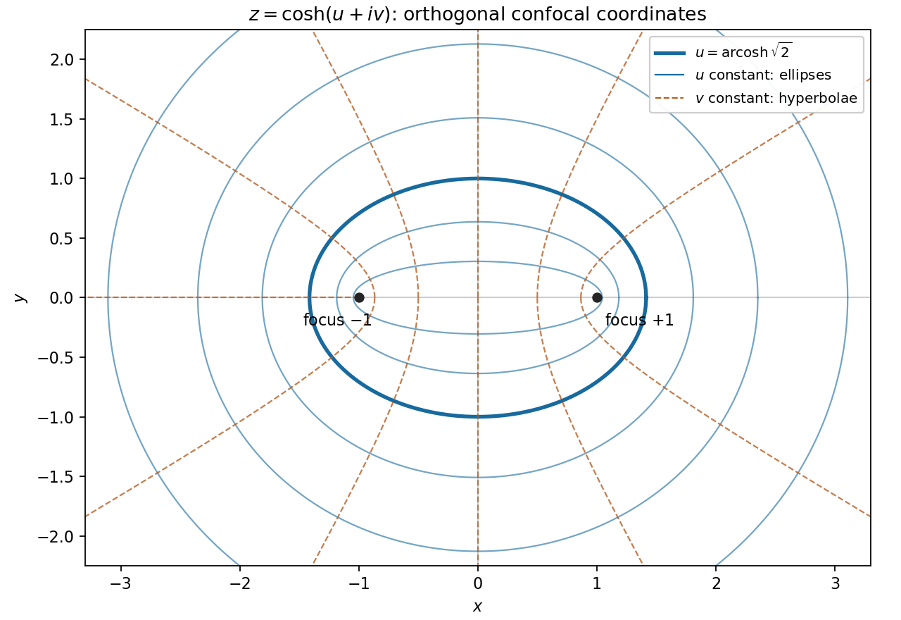
On the specified ellipse, the semiaxes are $\sqrt{2}$ and $1$, so its elliptic coordinate is $u_0=\mathrm{arcosh}\sqrt{2}=\log (\sqrt{2}+1)$. Thus in the exterior,is a harmonic function with a homogeneous Dirichlet boundary condition on that ellipse. Choose the square root with $\sqrt{z^2-1}\sim z$ at infinity. Although a global complex logarithm requires a cut, its real part $\log |z+\sqrt{z^2-1}|$ is well defined throughout the exterior and gives the same $\varphi$.

Expanding at large $|z|$ yields $z+\sqrt{z^2-1}=2z[1-1/(4z^2)+O(|z{|}^{-4})]$. ThereforeIn particular the potential grows logarithmically in the distance, in every direction at infinity. It is the exterior solution; no harmonic continuation through the focal segment in the ellipse's interior is claimed.

Use the Wirtinger derivatives ${\partial }_z=({\partial }_x-i{\partial }_y)/2$ and ${\partial }_{\bar{z}}=({\partial }_x+i{\partial }_y)/2$, for which $\Delta =4{\partial }_z{\partial }_{\bar{z}}$. Since $H$ and $G$ are holomorphic,The Laplacian has real coefficients, so taking real and imaginary parts provesThis is the complex analytic representation of biharmonic functions; $F$ itself is generally not holomorphic because of its $\bar{z}$ factor.

Set $y={\sum }_{j\ge 0}{a}_j{x}^j$ and equate coefficients in the power series. The constant coefficient gives $a_2=0$. For $m\ge 1$, the coefficient of $x^m$ givesThe square bracket is $(m+1)(m+2)$, so the recurrence relation is $a_{j+3}=a_j$ for $j\ge 0$. The initial conditions give $a_0=1$, $a_1=0$, $a_2=0$. Hence

Summing the geometric series givesThere is a particularly short verification using the product rule:Also $y(0)=1$ and $y^{\prime }(0)=0$. The radius of convergence of the series is one, set by the three complex cube roots of unity; the closed expression continues the solution beyond that disk wherever its denominator is nonzero. The real initial-value solution extends on the interval $(-\infty ,1)$.

Substitute $y=v{P}_n$ into the Legendre differential equation and expand using the product rule. The terms proportional to $v$ cancel because $P_n$ is itself a solution. What remains isMultiplying by $P_n$ identifies an exact derivative:The latter form is convenient for reduction of order on intervals where $P_n\ne 0$ and $x\ne \pm 1$.

Two integrations give the general reduction of order formulaThe integral is local on intervals avoiding zeros of $P_n$. A pole of the integral at an interior polynomial zero need not be a singularity of $y$: the product extends by reduction of order across a zero of the known solution. After a standard normalization the independent second solution is the Legendre function of the second kind $Q_n$.

For normalized Legendre polynomials, $P_n(1)=1$ and $P_n(-1)=(-1{)}^n$. Near the endpoints the integral factor has the asymptoticsandThus an independent solution, for which $C_2\ne 0$, has the logarithmic endpoint singularitiesThe constants are understood for a solution continued consistently across the ordinary interior points. Adding any multiple of $P_n$ cannot cancel these logarithms. This explains why boundedness at an endpoint selects the Legendre polynomial and excludes the independent Legendre function of the second kind.

Write $P_n(x)\sim c_n{x}^n$ with $c_n\ne 0$. For $n\ge 1$, this branch grows. Choosing the other reduction of order solution by an integral from infinity gives, on $x>1$,Thus for $n\ge 1$, every bounded exterior solution decays as $|x{|}^{-n-1}$, up to a constant factor, on each exterior interval. Equivalently the dominant-balance exponents in the Legendre differential equation are $n$ and $-n-1$.

There is an important exception at degree zero. Since $P_0=1$,These solutions are bounded even when $C_1\ne 0$; boundedness alone does not then imply decay to zero. The constants on $x>1$ and $x<-1$ are independent unless continuation across the singular endpoints is specified.

For a variation $y+\epsilon \eta$ with $\eta (a)=\eta (b)=0$, the first variation of the functional isThe boundary term vanishes by the fixed endpoints. The fundamental lemma of the calculus of variations therefore gives the Euler-Lagrange equation