[ref]
https://www.whatdotheyknow.com/request/natural_science_tripos_physics_e_2/response/2340776/attach/2/FOI%202023%20399%20Zahid%20materials.pdf?cookie_passthrough=1. Original public PDF, physical pages 72–78; dated 25 May 2013
In the small-angle approximation the physical pendulum is a harmonic oscillator with . Its classical energy is . Equating this to givesAn oscillating bob is not a single stationary energy eigenstate. An ideal coherent state has a Poisson distribution of oscillator occupations centred on this mean, with relative spread , exceptionally small here. This quantum occupation scale of a classical oscillator fixes the excitation scale without requiring the real, damped clock to be a pure coherent state.
The free particle dispersion relation is . HenceThe phase velocity follows constant-phase surfaces of a plane wave. The group velocity follows the envelope of a narrow-band wave packet and equals its classical velocity . Dispersion can spread the packet; the phase speed is not the particle's transport velocity. In three dimensions and the phase speed quoted is along .
The mass dependence of fixed-barrier tunnelling follows by holding energy and the potential-energy barrier fixed: quantum tunnelling has the leading WKB approximationThe alpha-particle mass is about electron masses, so its decay exponent is about 85 times larger for the same profile. Exponential suppression therefore makes transmission much smaller. This comparison holds the potential energy and incident energy fixed: the same electrostatic potential is not the same potential-energy barrier for charges of different magnitude and sign.
For the squared discrepancy of a digit frequency, write . The plotted ordinates are , , , , and in increasing . Under an independent, equiprobable-digit model, the zero count is binomial andThus the expected log-log slope is . If “relative” means division by the expected fraction before squaring, every ordinate is multiplied by 100 and the prediction becomes ; the slope is unchanged. These are nested prefixes of one digit sequence, so the points are correlated, rounded observations, not independent variance estimates. Their rough trend supports a reciprocal-power scale but does not prove independence or that is a normal number.
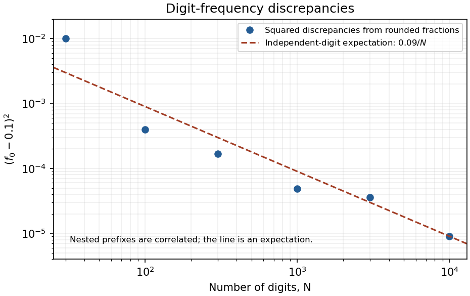
Original log-log plot of squared digit-frequency discrepancies with the independent-digit expectation
. Details. 
From Snell's law, . Treating the quoted angle errors as independent one-standard-deviation uncertainties and using radians in derivatives,This refractive-index uncertainty from Snell's law is first-order propagation of uncertainty, with air's index approximated by one. Correlated angular calibration errors add . If the quoted errors are hard bounds instead, their conservative first-order sum gives about , rather than the statistical quadrature value.
Apply the radial momentum operator to a smooth radial test function. More generally , giving the first two labelled identities. Expanding the square gives the third:The kinetic-energy decomposition is . A central potential commutes with and , so choose simultaneous angular eigenfunctions , with and . The radial Hamiltonian consequently has the stated centrifugal term. The radial inner product uses measure ; adjoints below are taken on compatible regular bound-state domains. The formal radial momentum is not thereby asserted to be a self-adjoint observable on a half-line.
Set , and . Since formally and ,The hydrogen radial Hamiltonian factorization follows by matching the Coulomb coefficient, which fixes the Bohr radiusFor the second pair of labelled relations, the opposite product changes the sign of , henceUsing in the factorization then givesThis Coulomb angular-momentum intertwining means applying to an energy eigenstate either gives zero or an eigenstate of with the same energy. For a normalized negative-energy state,At fixed this would become negative if raising continued indefinitely. The bound-state ladder termination by norm positivity occurs at some with , givingThe terminating radial function is proportional to , regular and normalizable; adjoint intertwiners generate lower values at fixed . Positive-energy scattering states are not subject to this terminating negative-energy argument. Here is the mass in the supplied Hamiltonian; including nuclear motion replaces it by the reduced mass.
The remaining cyclic commutators are and . In a spin- irreducible representation,For spin one-half, , appropriate to an electron's spin. Each , so this Hamiltonian is . The orthonormal vectors and are eigenstates with the same energy ; every normalized superposition is also an eigenstate. The term vanishes identically because spin-one-half quadratic anisotropy is constant.
For the supplied three-dimensional basis one consistent choice isThese Hermitian matrices obey the cyclic commutators with the given , and , representing spin one. Their squares giveThus the three normalized Cartesian basis vectors have energies , and , respectively; degeneracies permit arbitrary orthonormal choices in the corresponding eigenspaces.
The parallel and antiparallel states are and . Evolution from the first givesThis spin-one reversal under quadratic anisotropy is complete whenprovided . If , its initial state is stationary up to phase and complete reversal never occurs. Assume real for a Hermitian Hamiltonian.
The stationary equation isThe second derivative represents kinetic energy; the delta term is an attractive point interaction, with having dimensions energy times length. A jump in would produce a delta derivative in , with no matching term in this potential, so is continuous. Integrating through the origin givesFor define . Each side has general solution with independent constants. Square integrability retains on the left and on the right. The jump requires , and wavefunction normalization givesThere is one bound state for every .
For write . General solutions are independent combinations of and on each side. For incidence from the left choose and . Continuity gives and the jump gives . With ,The incident and transmitted velocities are equal, so squared amplitude ratios are current ratios here. At fixed positive energy, gives full transmission and increasing gives increasing reflection, approaching unity. Even an attractive point well reflects quantum waves; energy is conserved, and the static potential does not irreversibly capture the incident particle into its bound state.
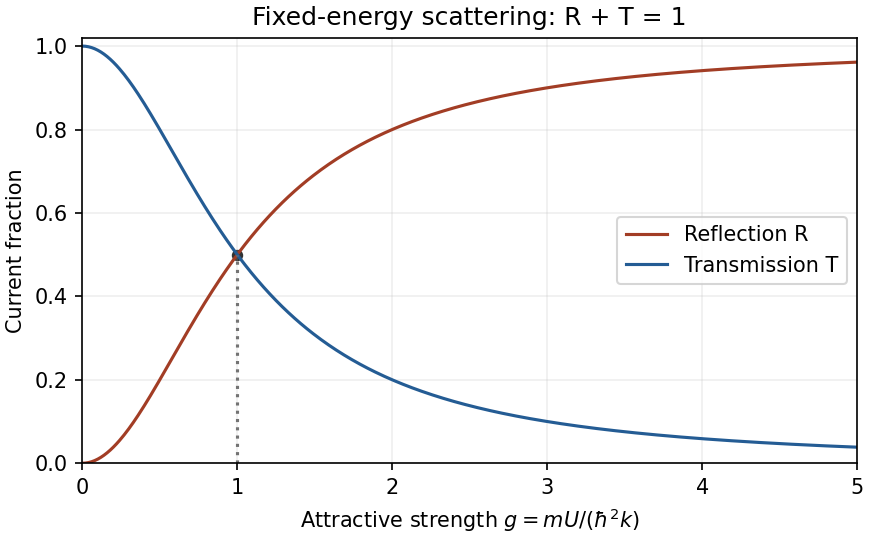
Original reflection and transmission curves versus dimensionless attractive-well strength at fixed incident energy
. Details. 
The anisotropic quantum harmonic oscillator is a sum of three commuting one-coordinate oscillator Hamiltonians. Substituting and dividing by gives a sum of three functions of independent coordinates, so each equals a separation constant. ConsequentlyFor a time-independent operator, conservation for arbitrary states follows from , since . The first labelled operator is ; the second is . The kinetic energy is rotationally invariant. The potential is invariant under rotations about precisely when (i) ; full rotational invariance requires (ii) . For positive oscillator frequencies these are equality of the frequencies themselves. Acting with the commutators on arbitrary test functions excludes anisotropic potentials in case (ii).
In the isotropic case let . ThenThe polynomial is the first excited oscillator factor and the other two factors are ground-state Gaussians. The first excited spatial level has three independent choices, proportional to . Odd parity gives , and Gaussian integration yieldsFor oscillator uncertainty and allocation of classical energy, the mode has energy , whose classical amplitude is , giving . If “same energy” instead means assigning the entire three-dimensional energy to one classical coordinate, its amplitude is and the ratio is . A general three-dimensional classical orbit's amplitude is not fixed by total energy without specifying its allocation among modes.
The capacity of an isotropic oscillator shell, including the two electron spin states, is electrons. Nine non-interacting electrons occupy shells as for . ThusThe least positive excitation promotes an electron by one oscillator quantum. Rearrangements within the partly filled degenerate shell remain ground states and cost no energy.
A pure quantum state is a unit ray in a complex Hilbert space: normalization fixes total probability, a common phase is unobservable, and superpositions retain relative phases. Observables are self-adjoint operators. For an ideal projective measurement with spectral projector , the Born rule gives and the Lüders rule gives conditional state . This preserves an eigenspace, not necessarily a unique vector when the outcome is degenerate. Between measurements, a closed system evolves unitarily according to . Composite systems use tensor products; quantum statistics additionally restrict identical-particle states. These are a framework supported by many experiments, not separate logical deductions from any one experiment.
In the photoelectric effect, monochromatic light illuminates a clean metal and a retarding potential measures the largest emitted electron kinetic energy. frequency controls the stopping energy, , while in the one-photon regime intensity mainly controls the emission rate. A threshold frequency and a stopping-energy slope support quantized energy exchange rather than gradual absorption of arbitrary classical-wave energy by each electron. Contact potentials, surface contamination, dark current and spectral impurities require controls. Robert Andrews Millikan tested the frequency–stopping-potential relation with careful surface and electrical control.[ref]
A Direct Photoelectric Determination of Planck's h by Robert Andrews Millikan. 1916, apparatus and stopping-potential measurements, §§2–5
The Stern-Gerlach experiment sends a collimated neutral silver beam through an inhomogeneous magnetic field onto a detector. The force is approximately in an appropriate strong-field electronic description. Two resolved components rather than a continuous classical orientation spread support discrete angular-momentum projections. Field-off beam profiles and magnetic-gradient/beam-width controls distinguish splitting from ordinary broadening. In the modern description the silver ground electronic state has ; the 1922 experiment preceded the electron-spin interpretation. Ideal sequential analyzers along different axes illustrate incompatible observables and state preparation, but were not the original apparatus.[ref]
Der experimentelle Nachweis der Richtungsquantelung im Magnetfeld by Walther Gerlach and Otto Stern. 1922; translated experimental setup and field-on/off deposition profiles
In the Davisson–Germer experiment, accelerated electrons scatter from a nickel single crystal and an angularly scanned collector measures the scattered intensity. Changing voltage and crystal orientation changes narrow diffraction maxima. The inferred wavelength agrees with , with nonrelativistic . vacuum, crystal cleaning, energy selection and background measurements matter: adsorbed surface gas can produce additional diffraction features. This supports matter-wave amplitudes and interference, with measured intensities related to their squared magnitude; it does not mean an electron must follow a classical orbit through the apparatus.[ref]
Diffraction of Electrons by a Crystal of Nickel by C. Davisson and L. H. Germer. 1927, abstract; apparatus and diffraction patterns
Together these experiments motivate quantized outcomes, wave amplitudes and probabilistic measurement while leaving a distinction between observed evidence and the general postulates used to organize it.A continuous symmetry is represented by a unitary family with a self-adjoint conserved generator of a continuous quantum symmetry . If for all , differentiating gives . Thus, for no explicit time dependence,translation invariance conserves the corresponding momentum component; rotational invariance about one axis conserves that angular-momentum component. A central potential conserves all components and , but the components need not be simultaneously measurable because . Time-translation invariance of a closed system gives a time-independent Hamiltonian and energy conservation.
A discrete symmetry need not have a continuously varying generator. For parity, lets stationary states be chosen even or odd, and preserves parity sectors. symmetry does not force every state to be an eigenstate of its conserved observable. Explicit time dependence adds to the conservation equation, and an external symmetry-breaking potential generally permits exchange with the environment. Degenerate eigenspaces require choosing a compatible common basis rather than assuming every eigenvector already diagonalizes every commuting operator.
For a dilute linear diatomic gas with fixed molecular number, translation contributes molar . Rotational levels are with degeneracy :At rotational excitation is frozen out; at the partition function is proportional to , giving and . Nuclear-spin populations and molecular symmetry modify detailed low-temperature behaviour. The high-temperature result corresponds to two quadratic rotational degrees of freedom; a nonlinear molecule has three and contributes .
For each independent harmonic vibration, write . Its energy and heat capacity areThe contribution is exponentially small at low temperature and approaches per mode at high temperature. zero-point energy does not contribute to . Typically rotations activate before bond stretching, producing diatomic plateaus as temperature increases within the molecular regime; ideal-gas . Dissociation, electronic excitation and nonideal interactions eventually invalidate this simple sequence. Polyatomic gases sum over their distinct vibrational frequencies; no single activation temperature describes all modes.
A black body absorbs all incident radiation; a small opening into an equilibrated opaque cavity approximates it because internal reflections strongly suppress escape without absorption. Equilibrium radiation has zero photon chemical potential. Counting electromagnetic modes and assigning mean occupation gives the spectral energy densityAt low frequency this becomes the Rayleigh-Jeans law, ; using that limit at all frequencies gives the ultraviolet catastrophe. At high frequency the exponential suppresses the spectrum. Quantized mode energy resolves the classical divergence.
Integration gives . An isotropic radiation field sends outward flux through a small aperture, soDifferentiating the wavelength spectrum gives ; the frequency-spectrum maximum is a different transformed peak, not simply . A real surface has emissivity less than one and possibly dependent on wavelength. Cavity temperature uniformity, aperture geometry, calibrated detector response and background subtraction are necessary when testing the spectrum or inferring temperature from it.
An ideal operational amplifier has infinite differential open-loop gain, infinite input impedance, zero output impedance and unlimited bandwidth and output capability, and zero input offset voltage and input bias current. In a stable negative-feedback circuit operating linearly, its input currents vanish and . This equality is a feedback consequence, not a rule for a saturated or open-loop amplifier. Here the grounded non-inverting input makes the inverting node a virtual earth.
The inverting two-pole band-pass filter has a series resistor and capacitor input, while the feedback arm is a parallel resistor and capacitor. With Laplace variable ,Kirchhoff's current law at virtual earth gives the minus sign. Substituting yieldsIt vanishes at zero and infinite frequency, with low-frequency and high-frequency . Differentiation gives the single maximumFor , the broad interval has . For , the interval instead has . The same rising and falling asymptotes apply outside either plateau.
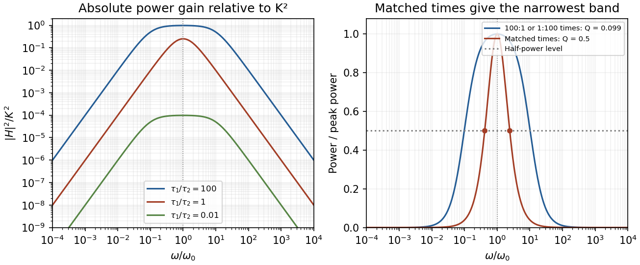
Original ideal filter power gains for different time-constant ratios, showing the finite selectivity limit
. Details. 
Writing and , the half-power frequencies and quality factor areEqual time constants give the narrowest fractional pass-band achievable here, with andThis topology cannot make a genuinely sharp, high- band-pass. Its poles are real, and the selectivity bound for a two-real-pole band-pass prevents arbitrarily narrow selection. A more selective resonant filter needs additional circuit structure. The gain above answers the component-ratio question for the sharpest available setting without assuming an impossible limit.
Real amplifiers have finite frequency-dependent gain and phase lag, so virtual earth becomes inaccurate, the response changes and stability must be checked. Gain-bandwidth limits, slew rate for large signals, output loading and amplifier saturation also matter. Component tolerances move the corners; capacitor parasitics, stray capacitance, resistor noise and input noise become significant. The ideal high-frequency tail should not be extrapolated beyond the amplifier and lumped-component operating ranges.
A systematic error shifts results in a reproducible or correlated way relative to the measurand. Examples include zero offsets, gain miscalibration, nonlinearity, drift, geometrical misalignment, loading, background contamination and an inadequate response model. Repeated measurements under unchanged conditions can reduce independent noise without exposing such a shift; a small standard error is not proof of measurement accuracy.
Use traceable standards and independent measurement methods, test zero and span, reverse the physical signal where possible, and vary the conditions that could cause the bias. For common-offset cancellation by signal reversal, take measurements and . The half-difference estimates while the half-sum diagnoses an unchanged offset . Drift between the two readings would violate that cancellation, so alternate or interleave measurements. Randomizing acquisition order separates slow drift from controlled parameter changes; blanks and calibration samples test backgrounds and instrument gain. Blinding helps reduce analysis choices that follow an expected answer.
Corrections have uncertainties and may be correlated across data. Include residual offsets and gains as nuisance parameters or propagate their calibration covariance, rather than treating a common calibration error as fresh independent noise for each datum. Document assumptions and check stability with controlled perturbations. These methods suppress or quantify specified systematic effects; they cannot guarantee elimination of every unknown bias.
The likelihood is considered as a function of parameters at the observed data. It is not itself a probability distribution over . Bayes' theorem givesThe prior represents parameter information before these data; the denominator normalizes the posterior and can compare fully specified models with compatible prior assumptions. Detector response, backgrounds, dependence and selection must be included in the data model.
For independent measurements with known errors, . Maximum likelihood minimizes this chi-squared and gives , . A Gaussian prior instead yieldsThis explicitly combines data and prior precision, approaching the weighted mean when prior information is weak. Unknown calibration parameters should be jointly inferred and marginalized, not silently fixed. posterior intervals are conditional on the assumed model and prior; posterior predictive checks and sensitivity to plausible priors help expose poor fits and weakly identified parameters. The maximum-likelihood estimate and a Bayesian posterior answer different inferential questions even when their numerical centres agree.
temperature changes alter dimensions, resistances, refractive indices and offsets; gradients can generate thermoelectric voltages. Identify the dominant heat paths and the experiment's temperature coefficients before choosing insulation. Reduce convection with an enclosure or, where appropriate, vacuum; reduce conduction through supports and leads with suitable geometry and thermal anchoring; use thermal radiation shields and low-emissivity surfaces to reduce radiative exchange. vacuum alone does not remove heat conduction through wires or thermal radiation.
In first-order thermal isolation, a sample with heat capacity and thermal conductance to its surroundings obeysThermal mass and insulation suppress rapid fluctuations but only delay slow ambient drift: the zero-frequency gain remains one. Active temperature control, a stable reference environment, adequate equilibration time and an appropriate sensor location address long-term stability. Self-heating produces a steady offset ; increasing insulation can worsen that offset and settling time. Check temperature gradients rather than relying on a remote thermometer.
Match materials or use differential/reference measurements to reduce expansion and resistance drift; keep dissimilar-metal junctions isothermal to suppress thermoelectric offsets. Log temperature alongside the signal and deliberately vary environmental temperature to measure residual coupling, using a physically justified correction with uncertainty. Interleave calibrations and allow equilibration after changing power. Feedback must remain stable, and heater/sensor electronics should not introduce electrical interference into the measurement.
Articles by others on the same topic
There are currently no matching articles.