Pressure and its physical terms. Solving the molar Van der Waals equation for pressure givesThe excluded-volume parameter reduces the volume available for translational motion, raising the kinetic pressure relative to . The attraction parameter lowers the pressure because attractive interactions reduce the momentum transferred to the boundary. This mean-field model treats as temperature-independent material constants. For one mole, is the sample volume with the molar amount already fixed; has units of that volume and of pressure times volume squared.
volume dependence of entropy. The Helmholtz free energy has differential . Equality of mixed derivatives yields the Maxwell relationFor this derivative is , givingEquivalently, with a common reference volume understood inside the logarithm. The equation of state fixes this volume dependence, not the otherwise unspecified function of temperature.
Excess entropy at fixed volume and temperature. The ideal gas has . ThereforeIntegrate from infinite volume, where the entropy difference is specified to vanish:It is negative because excluding configurations reduces the accessible state count. It tends to zero as and has leading dilute limit . This is the entropy excess of a van der Waals gas.
Effect of attraction. Restoring a temperature-independent changes the pressure by , but not its derivative with respect to temperature. With the same infinite-volume entropy reference, it therefore does not change at fixed . This can also be seen fromThe attraction affects internal energy and the equilibrium volume, so it can affect entropy indirectly when different state points are compared. If were temperature dependent, its derivative would contribute directly to the entropy; that is outside the stipulated constant-parameter model.
Coexistence isotherm. Below the Van der Waals critical point, the formal homogeneous isotherm has a local minimum and maximum. Its middle branch has , hence negative isothermal compressibility, and is mechanically unstable. Portions of the negative-slope branches can be metastable rather than globally stable. The equilibrium isotherm replaces the loop between liquid volume and vapour volume by a constant saturation pressure . The two volume are fixed byThe Maxwell equal-area construction expresses equality of the two phases' chemical potentials. Intermediate total volume are mixtures: changing the vapour fraction changes total volume at the same pressure, rather than following the unstable homogeneous curve. The spinodals are the turning points of the formal isotherm; they are distinct from the coexistence endpoints.
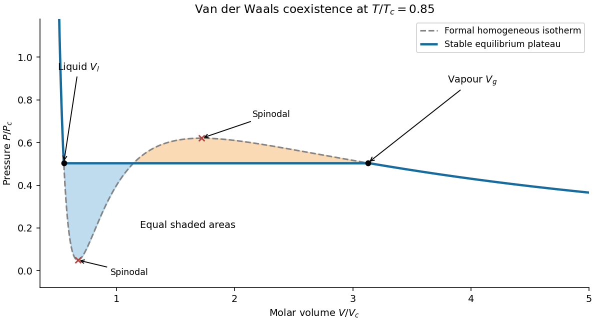
Original subcritical van der Waals isotherm showing the equal-area plateau, coexistence volumes and spinodals
. Details. Dense-phase volume at low temperature. At a general subcritical temperature, the two coexistence equations above must be solved together. For this equation of state the area condition is explicitlyThis supplies an exact implicit determination of the liquid volume even when a simple closed form is unavailable.
For the asymptotically low-temperature limit, put . The liquid is dense, , while the vapour is dilute, and . The area condition then givesThus the vapour volume grows exponentially in , and the saturation pressure is exponentially small. It is consequently consistent to neglect in the liquid equation to algebraic order in :Choose the root near , not the large-volume zero-pressure root:Expanding gives the leading requested dense-phase behavior,This is the low-temperature liquid volume of a van der Waals gas. Setting is an asymptotic approximation, not an exact coexistence condition at every temperature below . The figure illustrates generic subcritical coexistence; its finite-temperature liquid volume is determined by the full equal-area equations. The van der Waals liquid also ceases to be a realistic description at sufficiently low physical temperature, where other phases or quantum effects can matter.
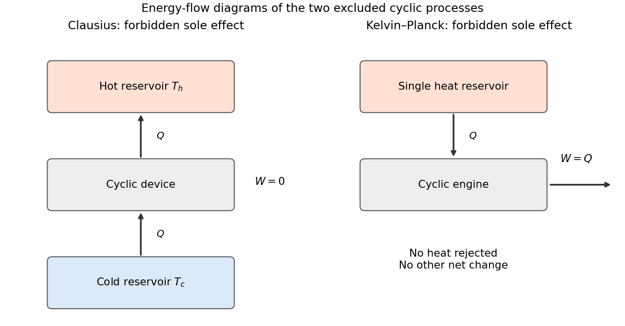
Two equivalent second-law statements. The Clausius statement of the second law forbids a cyclic device whose sole net effect is transferring heat from a colder reservoir to a hotter one. A refrigerator can make that transfer when supplied with work, so the sole-effect qualification matters. The Kelvin-Planck statement of the second law forbids a cyclic device whose sole net effect is drawing heat from a single reservoir and converting all of it into work. A heat engine can produce work when it also rejects heat to a colder reservoir.
The two statements are equivalent by combining a supposed violating device with an ordinary reversible engine or refrigerator: one can cancel one reservoir exchange and obtain a violation of the other statement. The following original schematic shows the forbidden sole effects, with arrows indicating energy flow.


Microscopic fluctuations. The second law is a macroscopic statistical law. A finite fluctuation can transfer a small heat amount from cold to hot, with reservoir entropy change . Such an individual event does not imply that a cyclic engine can extract systematic useful work from equilibrium. Entropy-decreasing trajectories become exceedingly improbable when the entropy involved is large compared with . Under suitable microscopic reversibility conditions, fluctuation relations quantify the relative probabilities of positive and negative entropy production and give nonnegative mean total entropy production. Thus a deterministic no-fluctuation reading has a limit at small scales or short times; the statistical second law remains applicable.
Maximum heating rate. Interpret the quoted as the maximum work-input rate to an ideal reversible heat pump. This interpretation is needed to obtain a heating rate larger than its electrical input; the wording does not explicitly distinguish input power from delivered heat. A reversible cycle satisfiesTherefore the heating coefficient of performance isWith and ,The additional heat comes from the outdoor reservoir; it is not produced by converting work into more energy than was supplied.
Lowest outdoor temperature. Let . The largest available heating rate is , while the house loses . Equilibrium can be maintained whenAt the limiting outdoor temperature,HenceThis is the indoor-temperature limit of a Carnot heat pump. It assumes the ideal pump retains its stated input-power capability over the operating range. Real heat exchangers require finite temperature differences and incur irreversibility, so the reversible result is an ideal upper performance bound.
Conventional heater. At this limiting outdoor temperature, the required delivered heating power is simply the house's heat loss:This is heat delivered to the house. The fuel-input power would be for heater efficiency . At the earlier outdoor temperature of , the required delivered heat would instead be ; the final question's reference temperature must be kept clear.
If is read literally as a maximum delivered heat rate rather than a work-input rating, the alternative answers are , , and a conventional heater delivering at that limit. Such a pump could not balance the stated house loss at . Both readings follow consistently once the ambiguous power rating is defined; the Carnot calculation above uses the work-input reading.
Configuration count. Choose the end-to-end direction as positive and let count rightward and leftward links. ThenA configuration is determined by choosing the positions of its leftward links, soThe counts must be nonnegative integers; in particular, allowed signed extensions occur in steps of . If distance means with neither direction selected, there are two corresponding sets for , adding a factor of two. That constant does not affect the tension. There is no excluded-volume penalty in this one-dimensional idealized count.
Entropy from the multiplicity. Put , so . Applying the leading Stirling's approximation to all three large factorials givesTerms subleading in , including logarithmic factorial prefactors, have been omitted consistently. Expanding near zero extension givesStretching reduces the number of available configurations and hence the entropy.
Tension and the range of Hooke's law. The model assigns no extension-dependent internal energy. At fixed temperature, the externally applied tension is . Differentiating the full leading entropy givesIt is the external force needed to oppose the chain's restoring entropic force. Only when can one put , yieldingThe paper's displayed linear law therefore requires this small-extension approximation, which is not explicitly stated in its premise . It is not the exact force law up to full extension. The entropic spring constant grows with temperature because stronger thermal disorder makes a given reduction in configurational entropy cost more free energy. This is the one-dimensional entropic chain force-extension relation.
A sparse number of backward links. Write , so and . Exactly,For fixed and large , each numerator factor approaches , givingMore precisely, the logarithm of the product is . A small relative error in the multiplicity requires ; merely need not make the omitted product close to one. The weaker sparse-link condition does suffice for the leading entropy density and leading high-extension tension. These are sparse backward links near full chain extension.
Tension in that limit. In the overlap regime , use Stirling also for :ThusThe full leading entropy would give , which has the same dominant logarithm when .
Approaching full extension. The continuum force law diverges logarithmically as , or . One must not literally apply Stirling to a zero factorial: at the discrete endpoint there is exactly one directed configuration, , and its entropy is zero. A continuous fixed-extension derivative is not defined at that endpoint.
An independent force-ensemble calculation makes the limiting physical statement precise. For applied tension , a link has partition function , giving the exact mean extensionIt approaches only as at positive temperature, and inversion reproduces the logarithmic force law for mean extension. In a real chain, bond extension or failure eventually replaces the ideal inextensible-link model.
Temperature as an equilibrium relation. Classical thermodynamics begins with the zeroth law of thermodynamics: thermal equilibrium is transitive. A thermometer can therefore assign a common empirical temperature to systems in mutual thermal equilibrium. Different thermometer properties initially give different monotone empirical scales; a resistance reading by itself does not define the absolute scale.
The Second law of thermodynamics provides a substance-independent thermodynamic scale. A reversible engine operating between reservoirs has a heat ratio depending only on their temperatures. One chooses absolute temperature so that , with the positive heat magnitudes. Its reversible efficiency is . Equivalently, reversible heat defines entropy through . For an equilibrium simple compressible system,Classical thermodynamics uses this relation without needing a microscopic account of entropy. A dilute-gas thermometer realizes an empirical scale approaching the thermodynamic scale after corrections for nonideal behavior.
Statistical meaning of the same derivative. In the microcanonical description, an equilibrium energy shell containing accessible states has . Its statistical temperature is consequentlyTo see why this is an equilibrium temperature, let two weakly coupled systems exchange a small energy while their total energy stays fixed. The combined multiplicity is . Maximizing its logarithm giveswhich is equality of the two inverse temperatures. Stability requires the total entropy maximum, not only stationarity. The overwhelmingly dominant macrostate in a large system therefore realizes the thermodynamic equilibrium condition.
A large reservoir gives a small subsystem the canonical probabilities , with . In that ensemble, and agree with macroscopic thermodynamic relations in their usual equilibrium regime. The equipartition identity for a classical dilute monatomic gas, , is a useful operational connection between microscopic motion and temperature, but is not a universal definition: quantum modes need not obey equipartition, and a system away from equilibrium need not have one temperature at all.
For finite systems one must specify the entropy convention and energy resolution; surface and fluctuation corrections can distinguish definitions that agree in the ordinary thermodynamic limit. Bounded-energy population-inverted systems can also have a negative entropy derivative and hence a negative statistical temperature. That possibility lies outside an ordinary positive-temperature ideal-gas thermometer; it does not mean temperature is merely an arbitrary average kinetic energy.
Obtaining the energy–temperature conversion. The Boltzmann constant connects entropy measured in with the dimensionless logarithm of a state count. Historically it could be determined from the ideal gas law : measure the molar gas constant and independently determine the Avogadro constant , then obtain . The independent particle-number determination matters; using alone would not fix energy per particle.
An electrical method uses Johnson-Nyquist noise. A resistor of resistance at known temperature has, in the classical range , a one-sided open-circuit voltage-noise spectrum . Over a calibrated flat bandwidth ,A practical measurement uses an equilibrium resistor, a calibrated low-noise amplifier and a known transfer function, subtracts or independently characterizes amplifier noise, and replaces a nominal bandwidth by the actual effective noise bandwidth. Varying temperature and fitting the mean-square voltage is more informative than treating one amplified voltage sample as the thermal variance. Other primary methods relate temperature to sound speed in a dilute gas or to calibrated particle diffusion and mobility.
There is a historically relevant unit-definition qualification: by the date of this exam, the revised SI had already taken effect on 20 May 2019. The kelvin is now defined by fixingThe same experiments now realize or compare thermodynamic temperatures using this fixed constant, whereas historically they measured the conversion constant on an independently defined temperature scale. The physical distinction between equilibrium temperature and microscopic state counting is unchanged.[ref]
https://www.bipm.org/en/measurement-units/. BIPM, SI definitions effective from 20 May 2019 and fixed Boltzmann constant
Articles by others on the same topic
There are currently no matching articles.