Taking the transpose gives , so is a symmetric matrix. For , has the standard normal distribution, whereas has the normal distribution . Distinct upper-triangular entries depend on disjoint sets of the original independent random variables, so they remain independent.
Consequently the joint probability density function, relative to , isHere because is a symmetric matrix. This is the Gaussian orthogonal ensemble, with off-diagonal variance one and diagonal variance two; the rescaled matrix has the corresponding off-diagonal variance.
We will also use its entry covariance. Expanding in the independent entries of , for which , givesThe symbols are Kronecker deltas. This formula includes the diagonal case, where the two terms both contribute.
The joint probability distribution of all entries of is unchanged by , so and have the same probability distribution. For the specified cyclic product , this transformation multiplies by . Every such product is an integrable random variable, since normal random variables have finite moments of all orders. Thus, for odd ,Repeated indices cause no difficulty: all factors change sign simultaneously. It would be incorrect to assume that these factors are independent.
The probabilistic form of Wick's theorem is Isserlis's theorem. If is a centered random vector with a multivariate Gaussian distribution and covariance matrix , its odd product moments vanish, and, for even ,Here is the set of perfect matchings of the labelled positions. The formula allows repeated coordinates and singular covariance matrices. To see the pairing rule, differentiate the moment-generating function once in each coordinate and set : only terms pairing all differentiated coordinates survive, each with the displayed product of covariances.
Take , with . These variables are linear combinations of the original independent normal random variables, hence are jointly Gaussian. They have zero means, soSubstituting the entry covariance from part (a)(i) identifies each parenthesis with , giving the requested identity.
The spectral theorem for real symmetric matrices identifies the sum of the th powers of the eigenvalues with the trace of the th matrix power. Therefore the moment of the empirical spectral measure isFor odd , every summand has zero expectation by part (a)(ii), so for every .
For the second moment, use . There are diagonal entries with variance two and ordered off-diagonal entries with variance one. Their means vanish, givingHence .
Write the four cyclic factors as , , and . The Gaussian moment pairing theorem gives three terms, corresponding to , and . We sum each term over .
For , the entry covariance givesIndeed the four products leave respectively three, two, two and one free indices. A cyclic relabelling gives exactly the same sum for .
For the crossing pairing ,The first product allows and freely, whereas each other product forces all four indices to coincide. Combining the three pairings and the trace normalization,
First , so the spectral theorem for real symmetric matrices gives real eigenvalues and an orthonormal basis of eigenvectors. Moreover, for every real vector ,Thus is a positive semidefinite matrix. For any nonzero eigenvector with eigenvalue ,This matrix is a scaled example of the Wishart distribution.
Let be row of , viewed as a real vector. These are independent standard Gaussian random vectors, and . The trace expression for the empirical spectral measure givesWe need the norm momentsFor completeness, has the chi-squared distribution with degrees of freedom. By independence and the Gaussian integral, its moment-generating function is for . Differentiating at zero once, twice and three times proves these three identities.
For the first moment,For the second moment, if , conditional expectation given gives , hence an unconditional value . Separating equal and unequal row indices yields
For the third moment, the summand is . There are three disjoint cases.
- If are all different, average over first. Its covariance matrix is the identity, so the conditional expectation of the last two factors is . The summand's expectation is therefore . There are such triples.
- If exactly two indices agree, cyclic symmetry reduces the calculation to . The product is , whose conditional expectation given is . Its expectation is , and there are such triples.
- If all three indices agree, the product is , with expectation . There are choices.
Let be the -by- evaluation matrix . The kernel evaluation matrix is the Gram matrix , so multiplicativity of the determinant givesBecause the polynomials are monic of consecutive degrees, their coefficient matrix relative to is a triangular matrix with unit diagonal. It has determinant one, so the Vandermonde determinant invariance under monic basis change givesSquaring removes the ordering sign. Thus the Gaussian unitary ensemble joint probability density function has precisely the kernel formNo orthogonality of the polynomials is needed for this step.
Use the inner product for a standard normal random variable . The degree-zero monic polynomial is . Write and . The conditionsuse and . Hence these first three Probabilists' Hermite polynomials areThe Gaussian fourth moment is , so their squared norms are
Gaudin's lemma is the projection kernel determinant integration identity. Suppose an integral kernel satisfieswith the relevant integrals absolutely convergent. Define and . ThenIn particular, a finite-rank projection kernel of rank has .
One can see the factor directly from the permutation expansion of the determinant. Terms whose permutation fixes integrate to . Every permutation on the other indices admits insertions of into a cycle. Each insertion reverses its sign, and the reproducing identity contracts its two adjacent kernel factors into one. These terms integrate to , proving the formula.
The squared norm of in is , where . Choose positive normalizing constantsThen are an orthonormal set for Lebesgue measure. Expanding the finite sums givesThus this is an orthogonal polynomial projection kernel, explicitlyThe positive constants above are forced by the reproducing identity: before normalization, its convolution multiplies each independent term by . Each multiplier must equal one. Changing the sign of a real leaves the kernel unchanged.
Use the symmetric joint probability density function of exchangeably labelled eigenvalues, normalized over all of . The finite-rank projection kernel hasSuccessive applications of Gaudin's lemma therefore giveIt follows thatAs a normalization check, the weighted Vandermonde determinant yieldsIf instead one uses ordered eigenvalues on , the normalized density on that chamber is six times the labelled density. In that convention the determinant prefactor on the chamber is one.
The correlation functions of a point process use factorial normalization:Start with . By Gaudin's lemma, integrating once gives , and integrating once gives . The factorial factors cancel, so the eigenvalues form a determinantal point process withandThe last equality uses the real symmetry of this kernel. In particular, and , as required for three points and six ordered pairs of distinct points.
Evaluate the orthogonal polynomial projection kernel on its diagonal:The terms cancel. Integrating against Lebesgue measure gives for a standard normal random variable , checking the correlation function of a point process normalization.
The correlation function of a point process is even and tends to zero as . Its derivative factors asConsequently its local maxima occur at , and its local minima at . The heights are
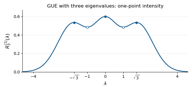
The three peaks of the GUE one-point correlation function
. Original plot of the exact correlation function of a point process calculated above. Filled markers indicate local maxima at ; hollow markers indicate the local minima at . The total area is three. Details.
For an interval , is the expected value of the number of eigenvalues in . Thus equally short intervals have the highest expected counts nearwith the central peak highest. Each exchangeably labelled eigenvalue has the same marginal probability density function . The three peaks should not be interpreted as three separate marginal densities for ordered eigenvalues.
In this case the most likely joint configuration also lies at these three positions. On the ordered chamber, the logarithm of the joint probability density function, up to a constant, isIts stationary equations are , satisfied by . For every nonzero real vector , the second directional derivative isThus is strictly concave on this convex chamber, proving that the stationary configuration is its unique global maximum. Permuting the labels gives the other maxima on .
The characteristic polynomial of the rotation matrix isIts roots are , soFor example is an eigenvector for and for . At or the two eigenvalues coincide; these events have probability zero under the uniform distribution.
The difference of the two eigenvalues is , hence . Its expectation isFor , put . The set of angles satisfying consists of , and , of total length . Thus the full cumulative distribution function isDifferentiating on gives the probability density functionThis is the arcsine distribution, equivalently the beta distribution with both parameters . It has no atoms at either endpoint.
Apply the same characteristic polynomial calculation with replaced by . Pathwise,The real-valued processes give continuous lifts of these angles. The eigenvalues coincide whenever ; the exponential formulas remain valid at those times.
Here . For , and . Since standard Brownian motion has quadratic variation , Itô's formula givesThereforeThe squared diffusion coefficient is . Its sign depends on : one cannot replace by the nonnegative square root while retaining the same driving Brownian motion.
The characteristic function of gives . Taking real parts and using ,There is also a direct check from the stochastic differential equation. Its Itô integral has zero expectation because its integrand is bounded. Thus satisfies and , whose solution is the same expression.
Interpret the source's missing variable in the limit arrow as . We prove convergence in distribution by showing that the angle of the Brownian motion becomes uniform on the circle group.
Let . For every integer , its angular Fourier coefficients satisfyThese are precisely the Fourier coefficients of the uniform distribution on the unit circle. Thus expectations of every trigonometric polynomial converge to its uniform angular average. By the Stone-Weierstrass theorem, trigonometric polynomials approximate continuous functions on the unit circle uniformly. Given an approximation error , the discrepancy of expectations is at most the polynomial discrepancy plus . Taking and then proves weak convergence of probability measures to uniform angular measure.
The function is continuous on the unit circle, so the continuous mapping theorem and part (a)(ii) implyEquivalently, the limiting arcsine distribution has cumulative distribution function for , and probability density function for . This proves the limiting law rather than inferring it merely from the limiting mean.
- Generate an -by- real matrix with independent entries having the standard normal distribution.
- Compute a QR decomposition with an orthogonal matrix and an upper triangular matrix.
- Put and return . Then with having strictly positive diagonal.
The matrix is invertible almost surely. Indeed, successively sampled Gaussian columns have probability zero of lying in the proper linear subspace spanned by the previous columns. Thus the diagonal signs used above exist with probability one. Equivalently, apply the Gram-Schmidt process to the columns, always dividing each residual by its positive Euclidean norm; this produces directly.
To prove uniformity, fix . Each column of has density proportional to , so orthogonal transformations preserve its probability distribution. Column independence therefore gives .
The QR decomposition with positive diagonal is unique: if , then is both an orthogonal matrix and an upper triangular matrix, hence diagonal with entries . Its diagonal entries are positive, so it is the identity. It follows that the orthogonal factor of is . ThereforeBy uniqueness of normalized Haar measure on the compact group , the returned matrix has exactly the required probability distribution. Reflection invariance gives each determinant sign probability , so the algorithm samples both components of the orthogonal group. The positive-diagonal correction is essential when a numerical QR decomposition chooses its own signs.
Articles by others on the same topic
There are currently no matching articles.