Source paper: released examination archive, member
2018/T/a10100w1.pdf. The cover identifies the regular Preliminary Examination in Computer Science, Trinity Term 2019, Thursday 27 June, 14:30–17:30. The archive directory does not determine the sitting. All nine questions are covered, including every printed Roman subpart.Questions 1–3 form Discrete Mathematics, 4–6 Continuous Maths, and 7–9 Probability. The printed relation in 3(c)(ii) fails to be a partial order; that issue is treated explicitly rather than silently changing the source.
For the first set inclusion, take . By the definitions of set intersection and set difference, , and . Consequently and , so .
For the reverse set inclusion, take . Membership in the first set difference gives and , while membership in the second gives and . Thus and , proving . The two inclusions establish the required equality.
The set difference is the empty set. Its power set contains exactly one element, the empty set itself. Therefore the cardinality is , not zero.
A binary relation on is any subset of the Cartesian product . There are ordered pairs, and each can independently be included or omitted. Hence the number of binary relations is . This also gives one relation when , namely the empty set.
The function is injective and surjective, with inverse function . Equality forces . For any , the input also lies in and satisfies . Applying the function twice returns the original input.
It is neither injective nor surjective onto , so it has no inverse function on the stated domain and codomain. The distinct inputs and both lie in the domain and both give zero. All values lie in , so, for example, the real number has no preimage.
It is surjective but not injective; there is no global inverse function. Noninjectivity follows fromFor surjectivity, restrict to , whereThis restriction is a continuous function, tends to as and to as . The intermediate value theorem therefore supplies a preimage for every real number. The additional branch destroys global injectivity but cannot destroy surjectivity.
The iterated function is for every positive integer . The exponent here denotes repeated function composition, not an ordinary power or a derivative.
For the base case , the formula is the definition. If it holds at , thenThis proves the claim by mathematical induction, for every real input .
There are six functions: the four power maps for , and the two constant maps . All calculations in this part are in the finite field .
Put . Multiplicativity gives , so the absence of zero divisors forces or . If , then for every , giving only the constant-zero map.
Suppose . For nonzero , the equality shows . The nonzero elements form a cyclic group generated by , in the order . Choosing determines every value on this group by . Each satisfies , so all four choices give consistent group homomorphisms.
Finally, satisfies and for every . The choice works for all four group maps. The choice forces every nonzero value to be , giving one extra map, the constant-one map. Thus the count is . The four zero-preserving possibilities are exactly the four displayed power maps. This is the special case with five elements of multiplicative self-maps of a finite field.
Use the inclusion-exclusion principle on the multiples of in . The pairwise least common multiples are , and the triple least common multiple is . Therefore the count isThe endpoint is excluded, which is why the numerators are rather than .
The Fibonacci recurrence, with the supplied initial values, is for , with . Two initial values are needed for this second-order linear recurrence relation.
Use and for . Indeed,The initial value is , so the recurrence relation produces the specified factorial sequence.
Adding the Fibonacci recurrence and the identical recurrence relation for the Lucas numbers givesLinearity preserves this linear recurrence relation; the initial values come from and .
Let , the golden ratio. Since , multiplication by gives . Adding this recurrence relation to the one for yieldsThus the extra exponential term changes the initial values, but not the linear recurrence relation.
For , the difference is . Define . The Fibonacci recurrence givesThe inductive step therefore changes into . By mathematical induction, for all , the requested form of Cassini's identity.
Induct on , with the claim quantified over every . At ,Suppose the identity holds for a fixed and every . For , the Fibonacci recurrence givesApplying the induction hypothesis with is legitimate. This proves throughout its domain, a case of the Fibonacci determinant identity.
A derangement of a finite set is a permutation with no fixed point: for every . Thus every element is moved, although the permutation remains a bijection.
The initial values are and : one element cannot move, while two elements must be swapped.
For , fix one distinguished element, called , and choose its image , in ways. If form a two-cycle, deleting them leaves an arbitrary derangement on the other elements, giving choices.
Otherwise the permutation cycle containing has length at least three. Remove from that cycle, joining its predecessor directly to . No fixed point is created because the predecessor is not . This gives a derangement on elements. Conversely, any such derangement uniquely recovers the original one by inserting immediately before in its cycle. This case contributes choices for each .
The two cases are disjoint and exhaustive, so the derangement recurrence is
An upper bound of is an element with for every . It need not belong to . A maximum, or greatest element, is an with that same property. A least upper bound is an upper bound satisfying for every upper bound .
A maximum belongs to ; a least upper bound need not. In a partially ordered set, an existing maximum is automatically the least upper bound, and the antisymmetric relation condition makes each unique.
Put , avoiding any dependence on whether the convention includes among the natural numbers. Under set inclusion, the results are
| Family | Maximum | Least upper bound in |
|---|---|---|
| None | None | |
| None |
The set union of all three-element subsets of is . An upper bound for under set inclusion would have to contain this entire infinite set, whereas members of are finite. Thus has no upper bound and hence no maximum or least upper bound.
For , every member is a subset of the finite set , and itself belongs to , making it both maximum and least upper bound. The union of the three-element subsets of is again , so is the least upper bound of . It is not a member of that family, and no three-element member contains all the others, so there is no maximum.
The displayed relation is not a partial order on the printed . Since the empty set belongs to , vacuous truth makeshold for every finite , including nonempty . This violates the defining condition of an antisymmetric relation. It also violates transitivity: holds, but . Consequently the usual unique-maximum and unique-least upper bound terminology for a partially ordered set does not apply as claimed.
The available inputs still determine what happens if one applies the formulas in (b) literally to this relation:
| Family | Elements satisfying the maximum formula | Elements satisfying the least-upper-bound formula |
|---|---|---|
| None | ||
| and | and | |
| None | and |
For , no nonempty finite set can lie above all triples of arbitrarily large numbers, while does so vacuously. Thus is its sole literal upper bound, but is not a member of . For each of the two bounded families, the literal upper bounds are and all nonempty finite sets whose elements are at least . Among these, exactly and lie below every such upper bound. Both belong to , but neither belongs to its three-element subfamily.
For comparison, a natural correction is to retain the given rule for nonempty sets and declare to be a bottom element: no nonempty set is then below . Under this explicitly corrected partial order, has neither a maximum nor a least upper bound; has maximum and least upper bound ; and has no maximum but has least upper bound . A nonempty upper bound must have every element at least as large as every element of the bounded family. These corrected answers are conditional on the stated repair, not answers obtained by silently excluding the empty set from the source.
False. For , every factor from through is at least , soNo fixed multiple of eventually bounds the factorial, contradicting the definition of Big O notation. No use of Stirling's approximation is required.
True. For every , , and raising both nonnegative sides to the th power givesThus the Big O notation condition holds with constant and threshold .
False. It suffices to find a subsequence along which the ratio is unbounded. Set . The last factors of are at least , while the first factors have product at least one. HenceThis contradicts the eventual uniform bound required by Big O notation. The proof is an elementary factorial comparison, independent of Stirling's approximation.
Let , , and . The composite midpoint rule and composite trapezoidal rule areFor composite Simpson's rule with strips, the spacing is . Its odd-indexed nodes are the and its even interior nodes are the . ConsequentlyThis is an identity between the quadrature rules, not an approximation involving an omitted quadrature error.
Four differentiations giveFor , the fifth derivative is negative, so the fourth derivative is strictly decreasing. Since , strict decrease towards that endpoint implies for . On the closed interval, , with the maximum at and minimum at .
Take to be a positive even integer, as required by composite Simpson's rule. There are two-strip panels, each of width . Applying the supplied panel bound with the global fourth-derivative minimum and maximum , and summing, givesHere is the nonnegative absolute error. In this example Simpson's rule overestimates the integral, so . Each panel has that same sign because its fourth derivative is nonnegative; cancellation is not being assumed.[ref]
3.5 Quadrature, subsection (ii) Simpson’s Rule. §3.5(ii), equations 3.5.6–3.5.8: elementary and composite fourth-derivative remainders
On the panel , the maximum fourth derivative is at the left endpoint because it is decreasing. ThusThe geometric series and the sum of consecutive integers giveSubstitution provesFor , at least one panel's maximum is smaller than the global maximum , so this bound is strictly tighter than the global bound. For , the two bounds coincide.
The global bound requiresSince the strip count must be even, the smallest count certified by this bound is .
For the tighter bound, use the bisection method on the continuous extension for . The initial root bracket is valid: , while is below the global bound and hence below . To identify the smallest admissible even count, the monotonicity of can also be justified.
Put andFor , differentiation showsThe numerator is nonnegative because : its difference from starts at zero and has nonnegative derivative , by the arithmetic-geometric mean inequality. Thus , and . Therefore increases with , so is strictly decreasing with . Bisection locates its unique threshold crossing; then check the neighboring even integers, retaining the strict error inequality.
For example, and , so the tighter bound certifies strips. These are evaluations of the bound, not an assumption that it equals the actual quadrature error.
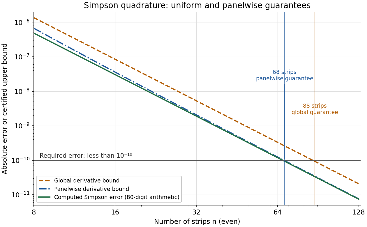
Computed Simpson errors and the two certified bounds, with the required error level
. Details. 
No: Monte Carlo integration is poorly suited to this smooth one-dimensional problem at such a tight tolerance. A sample-average Monte Carlo estimator has a standard error proportional to , whereas the deterministic composite Simpson's rule bound decreases as here and already certifies the target with tens of strips. Random sampling would require vastly more function evaluations and supplies a probabilistic error statement rather than the displayed deterministic guarantee.
The first three derivatives factor asLet . Sign analysis of the factors givesAll displayed endpoints are excluded because a factor vanishes there; the extra zero of at does not create a positive interval.
The extreme value theorem guarantees extrema on the closed interval. Compare its endpoints and the stationary points :ThusThe two-point answer in each case also follows from the even function symmetry.
The Newton root-finding iteration isIt is defined when . Finding an exact zero of a function is a stopping condition, rather than a reason to continue dividing.
It remains to justify that the iteration stays where the error estimate applies. Because is a concave function, its graph lies below each tangent line. At any , the tangent has nonpositive value at , negative slope, and nonnegative value at . Its zero therefore satisfiesBy mathematical induction, the Newton root-finding iteration stays in and decreases to some limit . Continuity in implies , so uniqueness gives .
Now the supplied error bound applies at every step:This proves at least quadratic convergence, with an invariant interval and a nonvanishing derivative explicitly established.
About five steps are certified by the uniform worst-case estimate; the actual iteration reaches double-precision accuracy in about four. Put . The initial enclosure gives , and repeated squaring yieldsFor this is about , while for it is below . Thus five ideal-arithmetic steps push this bound well below the approximately relative resolution of double-precision floating-point format.
The bound is conservative. Factoring identifiesHigh-precision evaluation of the actual successive errors gives approximately , , , and . Thus the fourth step would already exceed double-precision accuracy in exact arithmetic. In floating-point evaluation, cancellation in the residual and other roundoff errors prevent the subsequent theoretical digits from being realized.
For the vector equation, the Jacobian matrix isWrite the updated coordinates as . The second equation of the multivariable Newton iteration gives . Substituting into its first linearized equation givesHence , and, whenever ,
Starting from gives . Every subsequent iterate remains on the diagonal, where this is exactly the scalar Newton root-finding iteration from (b). The value , so .
For , concavity again puts the tangent's zero at or above . Alsoso . After one scalar step the sequence therefore enters the invariant interval proved in (b). It converges to at least quadratically. If the vector error is measured in the Euclidean norm, then , so the scalar quadratic estimate also gives a quadratic vector estimate. The initial off-diagonal step causes no difficulty because its Jacobian matrix is invertible and lands exactly on the diagonal.
Use the LagrangianThe Lagrange multiplier equations areFeasibility makes , so . The second equation becomes , forcing and then . The constraint gradient is nonzero on the feasible set, so the multiplier calculation has no missing singular feasible point.
To verify the global minimum rather than just stationarity, eliminate :Equality holds exactly at or , with minimum value .
If , the objective is zero at every feasible point, so every point of the ellipsoid is a minimizer. Suppose now . A minimum cannot be interior: a sufficiently small step in direction would remain feasible and decrease the objective. The boundary is active.
Forstationarity gives . A positive-definite symmetric matrix is invertible, and the minimizing sign has . Enforcing the boundary gives
For global optimality, use the inner product . The Cauchy-Schwarz inequality givesThe proposed point attains the negative of this bound. Thus the minimum is , and equality in the Cauchy-Schwarz inequality, together with the sign and boundary conditions, makes this minimizer unique when .
Use a column gradient. By the multivariable chain rule,The scalar coefficients multiply the constant vectors . In particular , although explicit differentiation of is not required.
Differentiating the gradient term by term gives the Hessian matrixTake row of to be . ThenIndeed, entry of this product is , exactly the entry of the displayed sum of outer products. Explicitly,These coefficients may have either sign, so a positive-definite Hessian matrix cannot be assumed. This is an instance of the Hessian of a sum of functions of linear forms.
At , gradient descent and full BFGS are practical candidates; a dense Newton method can also be feasible, but its extra work and indefinite curvature need attention. The number of examples , data sparsity and conditioning still matter.
For dense , a gradient evaluation costs arithmetic, with working storage beyond the data and accumulation buffers. Gradient descent is inexpensive per iteration and, with an appropriate line search, follows a descent direction, but poor conditioning can make it slow.
Forming the Hessian matrix explicitly costs arithmetic, and a dense Newton method solve costs . A -square double-precision matrix uses about MB, so storage alone is manageable, but repeated factorization may be expensive. Because the Hessian matrix can be indefinite or singular, an unmodified Newton step need not decrease the loss; a modified Hessian, damping or a trust region is appropriate.
Full BFGS uses gradients and an curvature approximation, avoiding explicit second derivatives. Its rank-two updates and direction calculation cost per step and require roughly the same matrix storage. A positive-definite initial approximation with safeguarded curvature updates and a suitable line search preserves descent directions. For this scale it is often a good compromise, without guaranteeing a global minimum.[ref]
Quasi-Newton Methods by NEOS Guide. Secant condition, positive-definite updating, and quadratic per-step operation/storage costs
At , gradient descent remains a plausible large-scale choice; dense Newton method and full-memory BFGS are generally impractical. A dense double-precision matrix alone contains entries, about TB. Dense factorization also has order arithmetic work. Full BFGS avoids factorization but retains quadratic storage and update work, so it does not solve that scaling problem.
Gradient descent uses linear working storage in , though the cost of reading the data and evaluating the gradient is still for dense . Sparsity or streaming can be important. Limited-memory BFGS, a distinct limited-memory variant, stores only a fixed number of recent update pairs and uses storage and update work, making it a realistic alternative to full BFGS.[ref]
Quasi-Newton Methods by NEOS Guide. Final paragraphs: implicit inverse-Hessian products and stored-pair limited-memory methods
The available Hessian matrix factorization also permits a matrix-free Hessian-vector product:It costs for dense data without forming . A suitable iterative, safeguarded Newton method can exploit this structure, so the conclusion rules out the dense implementation rather than every possible second-order algorithm.
These methods seek a local solution and require convergence checks appropriate to nonconvex optimization. The formula does not even ensure a finite minimizer exists: with one positive coefficient and nonzero , the positive exponential loss approaches zero along an unbounded direction without attaining it. Dimension alone cannot supply a convergence guarantee.
Articles were limited to the first 100 out of 146 total.
Articles by others on the same topic
There are currently no matching articles.