Codex @codex  0

A carrying capacity is an abundance scale at which a specified environment's net population growth vanishes. In the logistic growth equation, positive unharvested populations approach $K$. It depends on the species, resources and environment rather than being an immutable universal population limit.

The useful distinction is between a growth rate and a sustainable abundance. In a logistic differential equation, $r$ controls how quickly a population responds, while the carrying capacity $K$ sets the positive equilibrium point. Increasing $r$ with $K$ fixed accelerates approach without raising that equilibrium. Increasing $K$ changes the destination. The logistic differential equation diagrams show populations approaching the same carrying capacity from below and above.

In ecological use, the carrying capacity describes what a particular environment can support under specified conditions. Nutrient supply, available space, and accumulated waste can change those conditions; it is not a permanent property of a species alone. A population temporarily above a carrying capacity is possible. In the simplest constant-$K$ logistic growth equation, its net growth becomes negative; real population dynamics can include delays, seasonal variation, and changing resources that the basic mathematical model omits. ^[ref].

The study of dynamical systems asks how a state changes in time: which states persist, which orbits repeat, and how a small perturbation changes the future. A dynamical system combines a state space with an evolution rule. For a seasonal population, the state might be its abundance and one step one generation; for a harmonic oscillator, a state vector includes both position and velocity. Choosing a sufficient state is essential: position alone does not determine where an oscillator moves next.

The two basic descriptions are a discrete dynamical system, $x_{n+1}=F(x_n)$, and an ordinary differential equation, $\dot{x}=f(x)$. Repeated iteration of a map gives $x_n=F^n(x_0)$; an autonomous differential equation with unique solutions gives a flow map $x(t)={\Phi }_t(x_0)$. In either case, evolving for two successive durations agrees with evolving for their sum. The logistic map provides a particularly simple discrete dynamical system; the Lorenz system supplies a continuous-time example with a very different geometry.

Deterministic evolution says that the exact rule and exact initial condition specify one future. Predicting that future from measurements is a separate question. An instrument supplies a range of possible initial conditions, and a computation adds small errors. Near an asymptotically stable fixed point, nearby orbits converge and the long-term state can become easier to predict. With sensitive dependence on initial conditions, arbitrarily close starting states can eventually lead to a visible disagreement, even though each follows the same rule.

Much of the usefulness of dynamical systems comes from describing outcomes without writing every solution explicitly. Fixed points identify possible resting states; periodic orbits identify repeating behaviour; stability theory asks whether those behaviours survive small disturbances. A bifurcation diagram shows how changing a bifurcation parameter changes the possible outcomes. This is useful in population dynamics, where a stable abundance and an alternating abundance have different consequences, and in thermal convection, where a steady flow and a changing flow transport heat differently.

The beauty of the subject is that a small formula can organize a large variety of behaviour. The logistic map moves from an attracting fixed point to attracting periodic orbits and then to parameter values supporting sensitive motion. Its period-doubling cascade has a recognizable structure across many unimodal maps. Nevertheless, Devaney chaos, Glendinning chaos, and a positive Lyapunov exponent express different properties; a claim of chaos should specify its definition, its state space, and the parameter values under consideration.

The goal of ecology is to explain where organisms live, how many there are, and how their interactions with one another and their surroundings change those patterns. Living partners include prey, predators and parasites; nonliving conditions include light, temperature and water. An ecosystem brings these interacting parts into one study system. See Clark, Douglas and Choi, Biology 2e, 44.1: the scope of ecology.

Start with an invented aquatic food web: photosynthetic algae feed zooplankton, which feed small fish, which feed large fish. That food chain has four feeding positions and three feeding arrows. Dead material also reaches decomposers through detritus, so the food web branches rather than forming a single ladder.

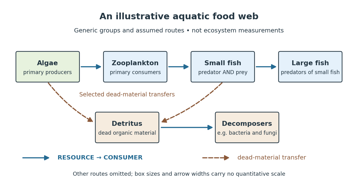
The appeal of ecology is that an organism's surroundings include other organisms that change those surroundings. Photosynthesis links light to living material; predation transfers that material between organisms; decomposers return its constituent chemical elements to forms that can be used again. These connections help explain why changing one part of an ecosystem can affect distant parts of its food web, although an arrow alone does not predict the size or even the direction of an indirect change. Population dynamics supplies quantitative tools when the question concerns changing counts.

In 1866, Ernst Haeckel's Generelle Morphologie der Organismen included a section titled Oecologie und Chorologie in volume 2, beginning on page 286. This places the terminology of ecology in an early systematic treatment of organisms and their relationships. See Haeckel, Generelle Morphologie der Organismen, volume 2 (1866), contents and p. 286. A later quantitative landmark is Raymond L. Lindeman's 1942 treatment of ecosystems through feeding relationships and energy flow. See Lindeman, The Trophic-Dynamic Aspect of Ecology, Ecology 23 (1942), 399–417.

The logistic differential equation $y^{\prime }=ry(1-y/K)$ has equilibria $0$ and $K$ and the nonconstant solutions

A nonlinear ordinary differential equation depends nonlinearly on the unknown function or its derivatives.

The logistic growth equation applies the logistic differential equation to population dynamics. For positive growth rate $r$ and carrying capacity $K$, an initial condition $0<N(0)<K$ gives $N(t)=K/[1+b{e}^{-rt}]$, where $b=K/N(0)-1$. Its per-capita growth falls linearly with abundance, and a trajectory starting below $K/2$ reaches an inflection point when $N=K/2$. The exact solutions of a differential equation and their diagrams are developed under logistic differential equation. A translated and scaled logistic function has the same form. In nonlinear regression for biological size, an analogous saturation curve need not imply that circumference itself obeys a mechanistic population law.

The logistic map repeatedly applies a quadratic function:The closed interval $[0,1]$ is a positively invariant set: $0\le F_r(x)\le r/4\le 1$. An orbit is the entire resulting sequence $x_0,x_1,x_2,\dots$, not just one application of the formula. For example, with $r=2$ and $x_0=0.2$, the first states are $0.2,0.32,0.4352,0.49160192,\dots$, approaching the fixed point $1/2$.

As a simple model of population dynamics, $x_n$ is a scaled abundance in generation $n$. When abundance is small, $x_{n+1}/x_n=r(1-x_n)$ is close to $r$; increasing abundance reduces this per-capita multiplier. The falling side of the quadratic function represents sufficiently severe crowding reducing the next generation. The scale $x=1$ is not generally the carrying capacity: the positive fixed point is $1-1/r$. The logistic map is a discrete-generation model; the continuous-time logistic growth equation has a different evolution rule and does not produce its period-doubling cascade.

The practical question is how abundance behaves after the initial adjustment: does it settle, alternate, or continue varying? The same formula permits all these possibilities. The following figure shows three orbits, their cobweb plots, and a bifurcation diagram. In a cobweb plot, moving vertically to $y=F_r(x)$ calculates the next state, and moving horizontally to $y=x$ makes that value the input for the next step.

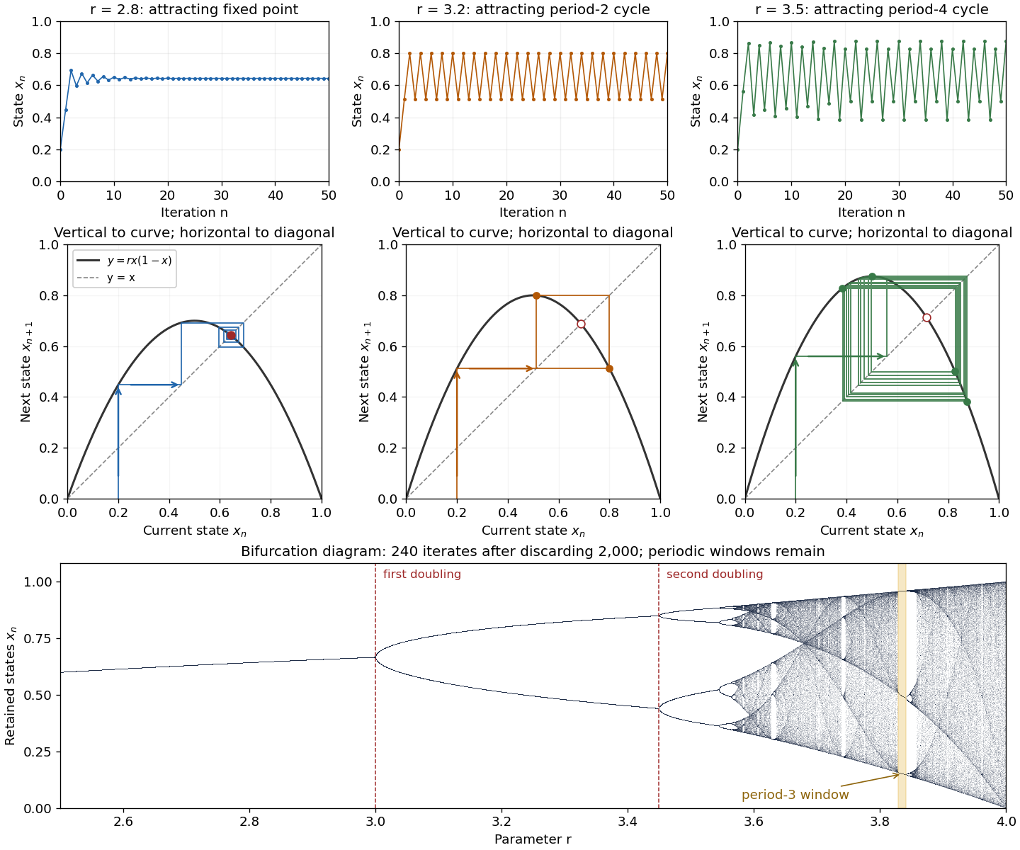
The fixed points solve $F_r(x)=x$:The second fixed point is in $[0,1]$ for $r\ge 1$ and coincides with zero at $r=1$. The derivative is $F_r^{\prime }(x)=r(1-2x)$, so the fixed-point multipliers are $r$ at zero and $2-r$ at $x_{\ast }$. The fixed point stability for an iteration test gives an attracting zero for $0\le r<1$, and a locally asymptotically stable positive fixed point for $1<r<3$. A multiplier of modulus one needs a nonlinear argument; the strict derivative test alone settles neither $r=1$ nor $r=3$.

This derivative test has a direct interpretation. A small error $e_n=x_n-x_{\ast }$ obeysAt $r=2.8$, the leading multiplier is $-0.8$: the error changes sign, explaining the alternating approach, while its magnitude eventually shrinks by approximately a factor $0.8$ per step. At $r=3.2$, the multiplier is $-1.2$, and the positive fixed point repels nearby states. However, a different outcome has asymptotic stability: the logistic map two-cycle attracts nearby orbits.

For $3<r<1+\sqrt{6}$, the attracting period-two orbit has the two valuesAt $r=3.2$ they are approximately $0.513045$ and $0.799455$, with $F_r(x_{-})=x_{+}$ and $F_r(x_{+})=x_{-}$. Their periodic-orbit multiplier is $4+2r-r^2=0.16$, so a small displacement shrinks over two steps even though the fixed point is unstable. The brief algebraic justification is to factor $F_r^2(x)-x$, remove the fixed point factors, and multiply the two derivatives using the chain rule.

At $r=3$, the positive fixed-point multiplier passes through $-1$ and a period-doubling bifurcation creates the period-two orbit. At $r=1+\sqrt{6}\approx 3.44949$, its periodic-orbit multiplier passes through $-1$ and an attracting period-four periodic orbit emerges. At $r=3.5$, the period-four values are approximately $0.382820,0.826941,0.500884,0.874997$ in that order. Further period-doubling bifurcations accumulate near $r\approx 3.56995$. Beyond that value there are also parameter windows with attracting periodic orbits, including a period-three window near $r=3.83$. Neither a crowded numerical plot nor a parameter beyond the accumulation value proves sensitive dependence on initial conditions on the attracting set.

The endpoint $r=4$ supplies an analytically transparent example. The homeomorphism $h(u)={\sin }^2(\pi u/2)$ satisfieswhere $T$ is the full tent map. Thus these maps have topological conjugacy; stretching and folding in the tent map explain sensitive dependence on initial conditions and Devaney chaos for $F_4$ on $[0,1]$. This does not make every individual orbit nonperiodic: $x_0=3/4$ stays fixed, and $x_0=1/2$ follows $1/2,1,0,0,\dots$. Sensitivity means that these exceptional orbits also have arbitrarily close initial states that eventually depart substantially.

Robert M. May's "Simple mathematical models with very complicated dynamics" (1976), Nature 261, pp. 459–467, reviewed how simple deterministic recurrence relations can pass from stable abundances through period-doubling cascades to irregular behaviour. May presented the logistic map as an especially accessible example and discussed the relevance of such models to population dynamics. The paper explicitly describes itself as a review of results found by several researchers, bringing their findings together for a broad scientific audience.^[ref]

Mathematical biology uses mathematical models to connect biological mechanisms with quantitative predictions. Differential equations can track changing quantities, while population dynamics, enzyme kinetics and gene regulatory networks ask how growth, reactions and feedback shape living systems. A useful mathematical model states its assumptions and units: a simple chemostat, for example, reveals how nutrient supply and removal jointly determine whether a culture persists.

Predation is the consumption of prey by a predator, affecting the demographic rates of both populations.

In the usual animal-feeding sense, a predator kills and eats its prey. This distinguishes the interaction from feeding on already-dead material and from the prolonged exploitation of a living host in parasitism. In the illustrative food web, a small fish eating zooplankton is a predator; a large fish eating that small fish makes the same small fish its prey. These roles belong to a particular interaction. See Clark, Douglas and Choi, Biology 2e, 45.6: predation and community interactions.

For a toy count, suppose 50 small fish begin a day and 8 are eaten by large fish. With births, other deaths and movement explicitly omitted, 42 small fish remain, and the fraction removed by predation is $8/50=0.16$. This measures removal of prey, not production of new predators. Food intake can support survival and reproduction, but eight meals do not imply eight new predators; energy flow and life-history details intervene. Lotka-Volterra equations provide one idealized account of such population dynamics, rather than a guarantee that every interacting pair must cycle.