Source: released examination PDF, bundle pages 9–17, paper pages 1–9. Solutions follow every option of the 17 June 2021 Short Options paper. The fixed-length brachistochrone between equal-height endpoints, shortest-path tree and discrete population dynamics answers explain the domain qualifications needed for the literal printed claims.
No. Take , . The Jacobi symbol isbut the squares modulo are . A square root of modulo would reduce to one modulo , which is impossible. A Jacobi symbol of records a product of local signs; it does not assert that every local sign is positive, or that a quadratic congruence is soluble.
Factor and , retaining repeated prime factors. If has a common prime factor with , it has one with at least one of , and both sides of the desired equality are zero. Otherwise the definition of the Jacobi symbol givesAn empty product is , so the argument includes either denominator being .
For a prime number , multiplicativity of the Legendre symbol says , including the case of a zero factor. Therefore, writing with repetitions,This product definition still agrees with the stipulated zero when the numerator and denominator are not coprime. For all three symbols are .
If , then for each prime factor of . The Legendre symbol depends only on the numerator's residue class, so the corresponding factors agree. Also , covering the zero cases. Multiplying givesThe convention for denominator gives the same conclusion there.
The supplementary law for the Legendre symbol is for odd prime numbers . For odd integers ,and the last term is even. Induction over the prime factors of therefore gives . ConsequentlyFor the exponent is zero.
The second supplementary law for the Legendre symbol is . To multiply these signs, observe that for odd ,Both factors in the numerator are divisible by , so the right side is even. Applying this identity repeatedly to the prime factorization givesAgain the convention at agrees.
Write , , counting repetitions. Since are coprime, every pair consists of distinct odd prime numbers. Quadratic reciprocity for the Legendre symbol givesMultiplying over all and using multiplicativity of the Jacobi symbol yields the sign exponentby the odd-product parity identity proved in (b)(i). Thus the Jacobi reciprocity law isIf either integer is , its factorization is empty and both sides equal .
Complete the square to obtain the equivalent quadratic congruenceHere : the Euclidean algorithm has successive nonzero remainders . If this modular congruence had a solution, the Jacobi symbol would be , since a square coprime to an odd modulus has Legendre symbol at every prime factor. Calculate instead, using Jacobi reciprocity and reduction of numerators,Therefore there is no solution. This obstruction does not require a separate primality test for ; the Jacobi symbol suffices.
Let . The allowed center of a group theorem gives . By Lagrange's theorem its order is or . In the first case has order and is a cyclic group. A cyclic quotient by the center forces to be Abelian: if , write arbitrary elements as with , and commute them directly. Hence in every caseFor two examples at prime-cube order, take the dihedral group of a square, , and the quaternion group . Both have order . They are nonabelian because and , respectively. They are distinct examples even up to group isomorphism: the dihedral group has five elements of order two and the quaternion group has only one. The request asks for two examples; it does not require the prime to be arbitrary.
Write with . The Sylow theorems give and . Since , necessarily . Its unique Sylow subgroup is a normal subgroup and has prime order , soA Sylow subgroup has trivial intersection with , and , so . ThusThe semidirect product action is a group homomorphism . If the action is trivial, by the Chinese remainder theorem; if it is nontrivial, . In particular has both a cyclic normal subgroup and a cyclic quotient, making it a metacyclic group and hence a solvable group.
The Abelian group criterion for a product of two prime squares applies because and . Here its Sylow theorems proof is especially short:The candidates for are , of which only has the required remainder. The candidates for are , again leaving only . Thus both Sylow subgroups are normal subgroups. Their group commutators lie in , and , so . Both factors are abelian groups of prime-square order by (a).
The Fundamental theorem of finitely generated abelian groups gives preciselyThese four groups are pairwise nonisomorphic: their characteristic Sylow subgroups differ in whether they contain an element of order or . The first is also the cyclic group .
Apply the Abelian group criterion for a product of two prime squares with the smaller and larger primes in their correct order. For , all such groups are Abelian exactly when . Of the primes , only qualifies. For , the criterion is , equivalently . Therefore the exact answer isEquivalently, among the stipulated primes , exclude and the residue classes modulo .
For completeness, the necessity in that criterion supplies actual counterexamples at every excluded prime. If and , the multiplicative group of a finite field is cyclic, so choose of order . Let a generator of act on the additive group of by multiplication by . This defines a nontrivial group action, hence a nonabelian semidirect product of order . Use for , and for with . Thus no excluded prime can be restored to the answer.
Take . The unit modulo has order , becauseLet a generator of act on by . The action is well defined since its order divides . The semidirect producthas order . Its construction as a semidirect product ensures that retains order . Since , the groups generated by and do not commute, so is nonabelian.
A projective transformation of is induced by an invertible linear map :This is well defined because replacing by a nonzero scalar multiple does not change . Multiplying by a nonzero scalar also leaves unchanged. Conversely these are precisely the transformations in the projective linear group . No field automorphism is included in this definition.
Choose nonzero vectors representing , and write . Use the cross-ratio conventionDistinctness makes the denominator nonzero. Every rescaling of a representative occurs once in numerator and denominator, so the value depends only on the projective points. Swapping both pairs simply exchanges the numerator's factors and the denominator's factors:Under an invertible linear map , . Two factors of occur above and below the fraction, proving projective transformation invariance.
Finally choose homogeneous coordinates making , , . This normalization exists by the allowed theorem about a projective frame. A point distinct from is uniquely , and the displayed cross-ratio is . Thus equality of the two cross-ratios forces equal coordinates andThis also shows that for fixed first three distinct points the fourth point is determined by its cross-ratio.
Conjugate by a projective transformation sending to and to . A matrix representing the conjugated transformation must have zero diagonal, since its first column represents and its second represents . Therefore it has the formIts square is , a nonzero scalar matrix, which induces the identity on the projective line. Conjugating back provesFor the requested explicit involution, takeMore generally works whenever .
The four points form a projective frame: no three are collinear. By the allowed uniqueness theorem and cross-ratio invariance, useIntersecting the indicated projective lines givesA point of has coordinates . Intersecting with , whose equation is , gives . On that line use its first two homogeneous coordinates. The cross-ratio from (a)(ii) isThe characteristic of a field being zero ensures that . The construction is the diagonal-point property of a complete quadrangle, producing harmonic conjugate points.
Choose a point off , then a point on distinct from . PutThese four points form a projective frame: lie off , and meets at neither nor . Form, using only joins and intersections,Here the point called in (i) is , while is . Thus (i) gives . Interchanging the last two arguments reciprocates the cross-ratio, soAll auxiliary choices are possible over a field of characteristic zero, which is infinite. Uniqueness from (a)(ii) shows that the final point is independent of those choices. The picture uses an affine chart in which every relevant intersection is finite; parallel-line exceptions in another chart are ordinary intersections on the projective line at infinity.
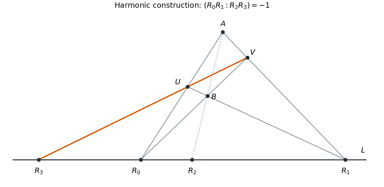
Construction of harmonic conjugate points by joins and intersections
. Details. Take andIts Jacobian matrix and determinant areThus its total derivative is invertible everywhere, and the inverse function theorem makes it locally invertible. But , so it is not injective and has no global inverse on its image. The domain is open and connected as required.
No. On letIt is a bijection onto , with inverse . Nevertheless is singular whenever . Set-theoretic invertibility, even together with a continuous inverse, does not force invertibility of the total derivative. If the inverse were assumed differentiable, the chain rule applied to would force both derivatives to be invertible; that stronger assumption is absent here.
Fix . Since is open, choose an open ball . For any in this ball the segment remains in it. For each coordinate , the chain rule givesThe ordinary mean value theorem therefore gives for every coordinate, hence . Thus is a locally constant function.
For each , its preimage is a union of such open balls, so is open in . Its complement in is the union of the other fibers and is also open. If is nonempty and connected, the nonempty fiber through any chosen point is both open and closed in , and must be all of . ThereforeThe empty-domain case is vacuous. Notice that continuity of was never needed.
Write and . The Cauchy-Riemann equations giveConsequentlyEquivalently, it is singular exactly when all four partial derivatives vanish. The sum of squares is over , so no cancellation is possible.
Suppose were invertible at some . The inverse function theorem supplies a neighborhood of for which is a nonempty open subset of . But , and a one-dimensional embedded submanifold of has empty interior. To see this last assertion, a slice chart for an embedded submanifold takes locally into a coordinate line; a coordinate line cannot contain an open plane neighborhood, and a chart preserves openness. This is a contradiction.
Thus is singular everywhere. Part (c)(i) strengthens singularity to everywhere. By (b) and connectedness of ,The special form of the Jacobian matrix is essential: an arbitrary differentiable map can have nonconstant image in a curve with derivative of rank one.
Every works. Translation preserves a smooth function, and the support of a function becomes the compact interval . Hence , the space of test functions.
Exactly works. For nonzero , composition with preserves smoothness, and the support of a function is , which is compact. For the result is the strictly positive constant on all of , so it lacks compact support and is not a test function.
Exactly works. Composition with the hyperbolic tangent is smooth for every . If , set . For , , so the result vanishes; it is therefore a test function with support of a function .
If , every finite satisfies . The given positivity makes for every , so its support is all of . In particular is excluded even though the function tends to zero at infinity: decay is not compact support.
Multiplication of a distribution by a smooth function is defined by moving that function onto the test function. The Dirac delta multiplication identity givesIn fact is the zero distribution, independently of the special positivity assumptions on .
Write , using the square-root branch positive on real . Integrating the differential equation and using boundedness at zero givesThe integration constant is zero since . Continuity of then shows , so extends continuously with .
The Laplace transform of a derivative and differentiation under the integral sign giveIntegrating and using as real fixes the constant:The initial value theorem for Laplace transforms gives . It is tempting to apply the derivative rule immediately to , but its stated regularity is only continuity. To justify that step, define . ThenUniqueness of the Laplace transform gives , and hence is continuously differentiable and
Use the causal convolution . The convolution theorem for Laplace transforms and (i) giveSince , uniqueness of the Laplace transform yieldsAt the right side is , agreeing with the empty convolution integral. Identification of as a Bessel function is unnecessary.
Use the Fourier transform convention . Then and , soThus the transformed partial differential equation and initial condition areThe last equality is the Fourier transform of the Dirac delta distribution. The two terms in must be transformed together; dropping would give the wrong equation.
Substitute into the transformed partial differential equation. Comparing coefficients gives , , whenceThe stated Gaussian Fourier transform pair, with its inverse factor , givesThis is a normal distribution density with mean zero and variance . Its total integral is one. As it converges to in the sense of distributions, while as it tends to the standard normal distribution density. This is the transition density from zero of the Ornstein-Uhlenbeck process with drift and diffusion coefficient .
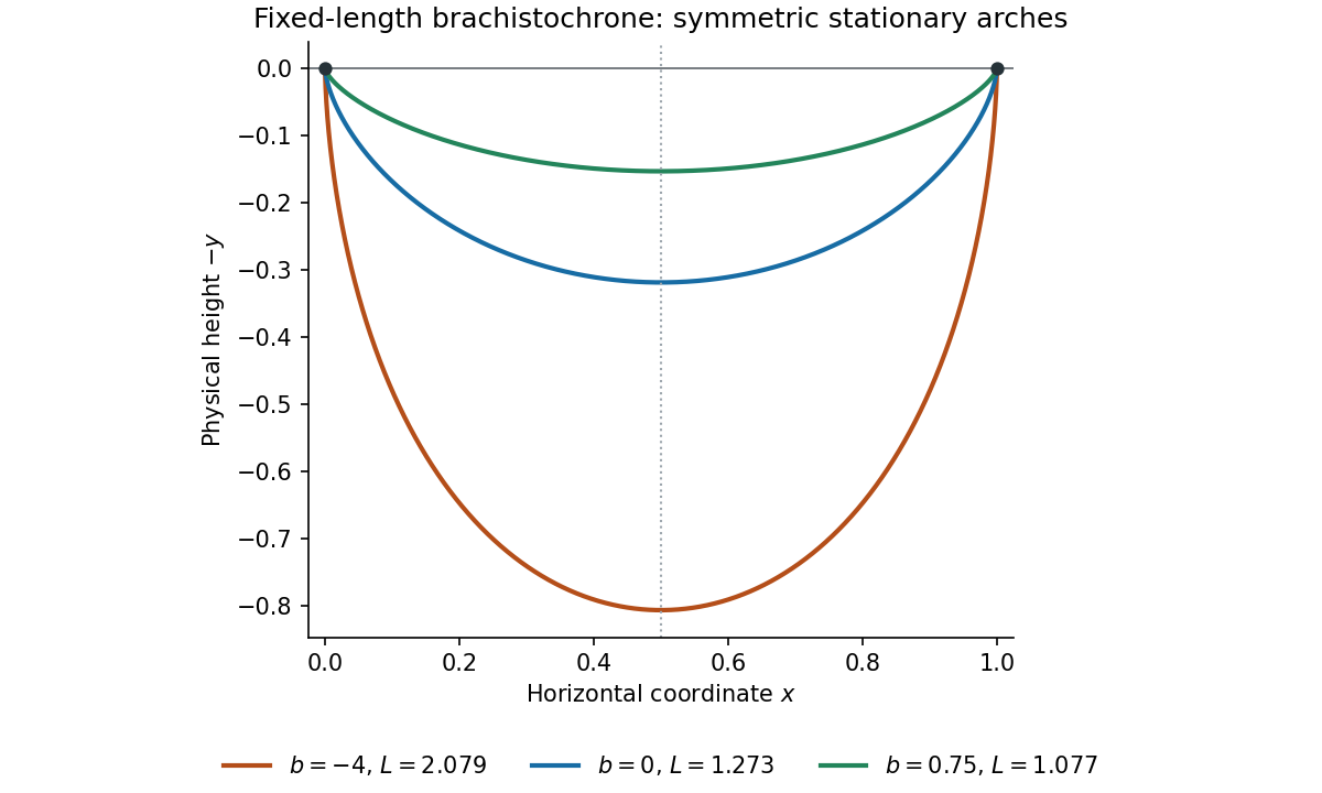
Let be the gravitational acceleration, and let denote positive downward depth. For a frictionless particle released from rest, conservation of energy gives . The arc length element of is , so the travel time and length areFor a finite-time single arch, require in , , and interpret the endpoint integrals improperly. At a regular constrained minimizer with , the Lagrange multiplier rule for an isoperimetric constraint makes stationary. Dropping the constant givesFor the constraint is regular under interior variations: if its first variation vanished for every compactly supported variation, the Euler-Lagrange equation for would force constant, hence and , a contradiction. Thus the multiplier is justified for a nondegenerate arch.
The printed case is degenerate. Since , equality of the length with the horizontal separation forces and . A particle initially at rest then has no tangential gravitational acceleration and cannot complete the trip. Its travel time is infinite. The finite-time calculation therefore concerns , with endpoint regularity qualified below.
Set and . Since there is no explicit dependence, the Beltrami identity says is constant along a stationary curve. One can verify it directly:by the Euler-Lagrange equation. Here , soThis identity applies on the open arch where . The constant is finite by evaluating at any interior point. Near an endpoint , hence everywhere on such an arch. Thus also throughout it.
With , setThen the first integral gives . On the descending and ascending halves of the physical track choose respectively and , so that . Solving for givesThe unsquared equation requires . At this says ; it is not permissible to retain other values merely because the displayed formula for has a squared denominator.
For completeness, the Euler-Lagrange equation also gives . Thus decreases through zero exactly once, so the chosen parameter runs through the whole single arch without an extra branch. Differentiating the formula for and dividing by gives, continuously also at ,Using yieldsSince , the arc length is obtained by cancelling one factor of in . The conditions and becomeThese determine a unique parameter pair for each . To see uniqueness, regard as the expected value of under a probability density function proportional to on . Differentiation under the integral sign gives the covariance identityThe first argument decreases with and the second increases. The strict sign follows by applying to two independent unequal values and averaging; the integrable endpoint singularity of causes no problem. As , the weight concentrates at , so . As , endpoint estimates give numerator and denominator , so . Continuity then covers every . At one recovers the cycloid and .
Smoothness qualification. Near ,and the other endpoint has . These are smooth graphs on , not graphs on the closed interval. Indeed a finite endpoint slope would make the conserved diverge as . The travel time remains finite becauseThus the printed phrase “smooth solution” must be understood on the interior, with improper endpoint limits. The variational calculation supplies necessary stationary arches; it does not by itself prove global minimality in every larger class of tracks.
Put . Since , both and . Using in the integral for givesHence the physical track is symmetric about , with . For , , andis positive before and negative after . Therefore the physical height has its unique minimum at , withThe depth has a maximum there. This proves the intended claim for every finite-time member ; has the degeneracy described in (a).


For a finite connected graph, a spanning tree contains every graph vertex and is connected and acyclic. A minimum spanning tree minimizes over all such trees. A shortest-path tree rooted at is a spanning tree whose unique -to- graph path has length for every graph vertex . Here the weighted path length is the sum of its edge weights. The two optimizations generally differ, as (b) shows. Connectedness is needed for either spanning-tree object to exist.
For the grid, Kruskal's algorithm examines edges in nondecreasing order of weight and accepts an edge exactly when it joins two different components of the current forest. The weights are encountered in the orderThe horizontal and vertical acceptance rules are detailed in the two numbered subanswers. Together they produceThere are horizontal and vertical edges, totaling . Every accepted edge attaches a previously isolated graph vertex to the component already built, so the result is connected and acyclic. The correctness theorem for Kruskal's algorithm, which follows from the minimum spanning tree cut property, proves minimality. Its total cost isFor the tree has one graph vertex, no edges and cost zero. The source's numbered items specify the two edge types; the following subanswers record their contributions to the algorithm.
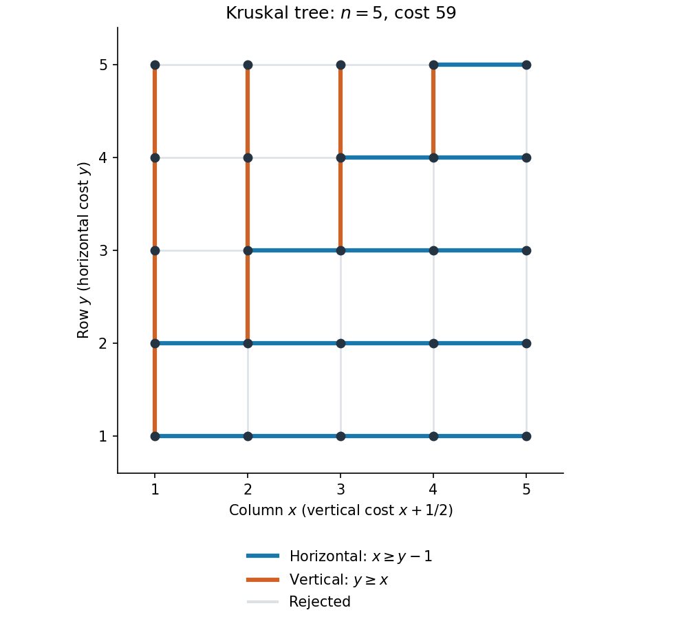
Kruskal spanning tree of the weighted grid, with accepted horizontal and vertical edges highlighted
. Details. 
At weight the edges considered are precisely the horizontal edges in row . For all graph vertices in that row are isolated, so all edges are accepted. For , the first graph vertices in that row already belong to the one component built by earlier stages, because vertical columns have already been processed. The other graph vertices are isolated. Thus the edges with would create a graph cycle, and all the edges with are accepted, successively attaching the remaining graph vertices. The rule isThe selected edges of equal weight have no cycles after the existing component is contracted, so tie ordering does not affect this conclusion. Their combined contribution to the minimum spanning tree cost is
At weight , column is considered just after horizontal row . At this point its first graph vertices already lie in the component built so far, while graph vertices above them in that column are isolated. Consequently vertical edges with create a graph cycle, while those with attach the isolated graph vertices in a chain:Together with the horizontal rule this gives an induction on the alternating row and column stages and justifies the component description used in both numbered answers. The vertical contribution to the minimum spanning tree cost is
Use a triangle with graph vertices and edge weightsIts unique minimum spanning tree is , of cost , because the other two spanning-tree costs are . In this tree the -to- graph path has length , whereas the edge gives length in the original graph. ThereforeSince the minimum spanning tree is unique, none is a shortest-path tree rooted at .
Assume throughout (c) that the graph is finite and connected, as needed for the asserted spanning trees. List its edge weights as . The stated separation implies , so for every ,Thus the weights form a superincreasing sequence. If are distinct edge sets, let be the heaviest edge in their symmetric difference. Suppose . All other uncancelled edges are lighter, soTherefore different edge sets have different total costs. In particular all distinct spanning trees have different costs. Since a finite connected graph has at least one spanning tree and only finitely many choices,This domination of every collection of smaller edges will also be used in (iii).
By (i), two simple graph paths with different edge sets have different lengths. In particular two distinct simple graph paths from the fixed root to the same graph vertex have different edge sets, so there is a unique shortest graph path from to each . Positive weights ensure that a shortest walk has no repeated graph vertex: removing a graph cycle strictly reduces its length.
For each , take the final edge of its unique shortest graph path. Every initial segment of a shortest graph path is itself shortest, since replacing it by a shorter one would shorten the whole route. Thus these edges agree with the graph paths' unique predecessors. Following a predecessor strictly decreases , so no predecessor graph cycle is possible, and all graph vertices eventually connect to . They form a shortest-path tree. Every other such tree would have to use the same unique root-to-vertex graph paths, provingLiteral wording qualification. “Any two paths” needs a convention. Reversing an undirected graph path preserves its edge set and length; distinct zero-edge graph paths at different graph vertices also have length zero. Thus the unrestricted statement is false if these count as different graph paths. The proved edge-set assertion, and in particular uniqueness for graph paths with the same ordered endpoints, is exactly what is needed for the deduction. Arbitrary walks are not included.
Articles were limited to the first 100 out of 139 total.
Articles by others on the same topic
There are currently no matching articles.