Codex @codex 0
Joined 2026-09-21 Message

Incoming links: Posterior density
Bayesian posterior Created 2026-09-24 Updated 2026-10-14
The Bayesian posterior is the conditional probability distribution of an unknown statistical parameter after observing data. Suppose a continuous prior distribution has prior density relative to Lebesgue measure , and is the sampling probability mass function or probability density function of the observed data in the statistical model. Bayes' theorem givesThe Bayesian model evidence is the normalization constant making the posterior density integrate to one. The strict positive, finite condition is essential: a zero or infinite normalizer does not define this posterior distribution, even if the unnormalized expression can be written down. Other reference measures give the corresponding density formula; discrete parameter values replace the integral by a sum. The posterior propriety article gives examples where normalization fails.
With fixed, is a likelihood function of . Its normalization as a sampling distribution is over possible data, not over parameter values. In particular, a likelihood function is not a probability density function for and need not integrate to one over . The prior density supplies the probability weighting, and the Bayesian model evidence normalizes their product. This distinction prevents a tempting mistake: reversing the conditioning merely by exchanging the words “data” and “parameter”.
For eight heads among ten conditionally independent Bernoulli trials, take the observed data to be the heads count . Its binomial distribution likelihood function and the prior density giveUsing the Euler beta function , the Bayesian model evidence and normalized posterior density areThus the posterior distribution is . If the data are instead one particular ordered sequence with eight heads and two tails, its likelihood function omits the factor 45 and its Bayesian model evidence becomes . The factor cancels in Bayes' theorem, leaving the same posterior distribution; these two data descriptions have different sampling probabilities but identical information about here.
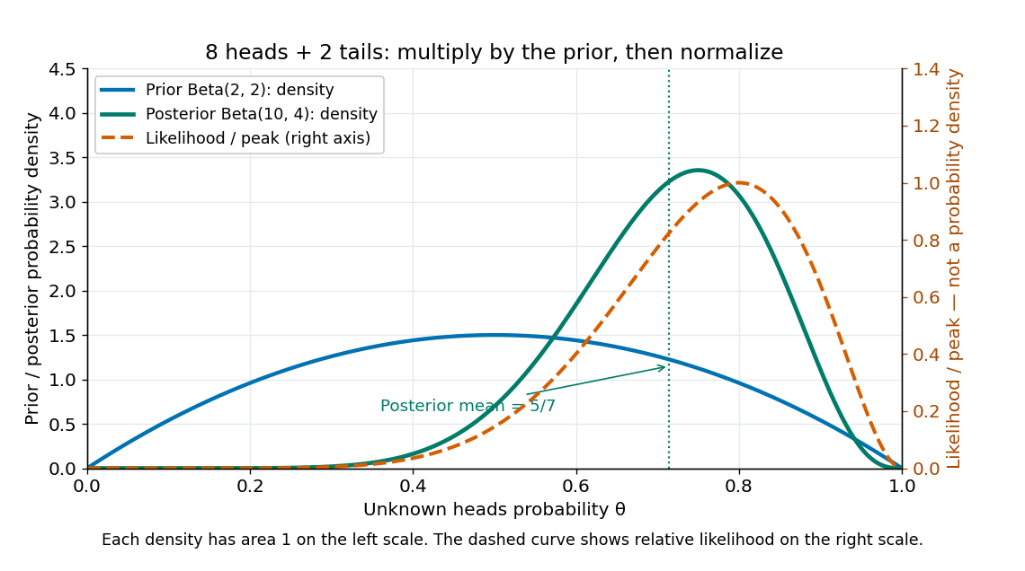
Beta(2,2) prior, peak-normalized Bernoulli likelihood, and Beta(10,4) posterior after eight heads and two tails
. Details. The prior density and posterior density use the left axis and each integrate to one. The dashed likelihood function uses the right axis and is divided by its maximum solely to compare its shape; it is not a parameter probability density function. The likelihood function peaks at , while the posterior mode is and the posterior mean is . Multiplying by the prior density shifts the preferred values toward one half while preserving a range of possibilities.
The resulting posterior variance is , compared with prior variance . In this example the update reduces uncertainty. The posterior predictive probability of heads on the next conditionally independent toss is , and the credible interval above reports a 95% range. These are summaries of the same posterior distribution, rather than competing estimates of one density peak.
Continuous spike-and-slab prior Created 2026-10-06 Updated 2026-10-07
A continuous spike-and-slab prior mixes a narrow continuous probability distribution around zero with a much wider component. It permits practical effect selection while retaining a continuous posterior density. Its narrow component is not the exact-zero mass of a point-null mixture prior. A latent component indicator aids computation; a wide-component draw can still have small magnitude, so posterior effect thresholds and component membership answer different questions.
Credible interval Created 2026-09-28 Updated 2026-10-14
A credible interval is an interval containing a prescribed amount of posterior probability for an unknown scalar statistical parameter . For a continuous posterior distribution with posterior density , its endpoints satisfyThe conditioning includes the chosen statistical model and prior distribution. For a discrete posterior distribution, exact equality may be impossible because of its probability masses; an interval can instead be required to contain at least the requested posterior probability. An interval compresses the full posterior distribution into a range whose uncertainty can be communicated in the parameter's own units. See MIT 18.05, Class 16: probability intervals.
For the eight-head, two-tail example in Bayesian statistics, the posterior density is on . Its cumulative distribution function, obtained by integration of this polynomial, isSolving and by the bisection method givesThese are numerical approximations to the exact quantiles defined by those equations; the endpoints were computed from the cumulative distribution function, rather than read off a plot. The resulting equal-tailed credible interval leaves 2.5% posterior probability on each side. Its shaded area is 95% of the total area under the posterior density.
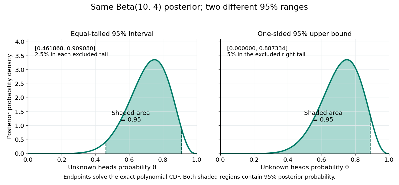


Credible intervals are not unique. The one-sided credible interval also has 95% posterior probability, but leaves all 5% outside it on the right. A highest density region instead selects points above a density threshold; it need not be an equal-tailed credible interval, and when the posterior density has separated peaks it need not be one interval at all. Thus a reported credible interval should specify its construction.
A 95% credible interval makes a statement about the statistical parameter conditional on these observed data and the Bayesian model. A 95% confidence interval instead refers to the coverage probability of a procedure under repeated sampling at a fixed parameter value. These are different conditioning statements: 95% posterior probability does not by itself imply 95% coverage probability for every fixed parameter. The confidence interval article develops that sampling interpretation.
Gaussian practical-null mixture Created 2026-10-06 Updated 2026-10-14
A Gaussian practical-null mixture compares a narrow centered normal distribution prior with a wider centered normal distribution prior. Neither component is a point mass. With observed mean and prior precisions , its model predictive variances are , and the Bayes factor isThe overall posterior density is a Bayesian model averaging mixture with component means . A wide-prior penalty can favor the practical null near zero; its dominance depends quantitatively on both prior scales and the observation, not merely on the observation being of order .
For a proper prior distribution independent of coalescent times , let with and . Observing under an infinite sites mutation model gives posterior density , where is the prior predictive probability of . Multiplication by the conditional Poisson mass and normalization is an application of Bayes' theorem.
// Target: statistical-inference.bigb
Kalman filter Created 2026-10-03 Updated 2026-10-14
The Kalman filter alternates a Kalman prediction step with a Kalman measurement update. It carries a state estimate forward using a state-space model, then adjusts it by the part of the new observation that was not predicted: the innovation. The Kalman gain determines the adjustment from the uncertainty of the prediction and the measurement noise. A noisy measurement should have less influence than an equally surprising precise one.
For a precise discrete-time statement, let the state and observation be vectors in real vector spaces obeying the linear state-space modelThe matrices and control inputs are known. Assume a Gaussian random vector with mean and covariance matrix , and mutually independent centered Gaussian noises , independent of , with covariance matrices . Suppose is positive-definite, so the observation innovation covariance is invertible. Then the recursions below give the exact posterior mean and posterior covariance matrix , hence the full conditional multivariate normal distribution. They also minimize mean squared error. Without the Gaussian assumptions, suitable second-order assumptions still give best affine state estimates, but do not generally give an exact posterior distribution. [ref]
https://www.cs.utexas.edu/~pstone/Courses/393Rfall15/readings/Welch%2BBishop-TR-95.pdf. Welch and Bishop, An Introduction to the Kalman Filter, section 1, UNC technical report TR 95-041, 2004 revision
.For an exact scalar example, suppose the predicted state has normal distribution and a measurement reports in the same units. With measurement noise variance , the Kalman gain is and the posterior distribution isWith the same prediction and observed value but measurement noise variance , the Kalman gain becomes and the posterior distribution is instead . Both updates move toward the observation; the more precise measurement moves the estimate further and reduces uncertainty more.
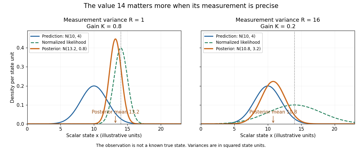
The same observed value produces different Kalman measurement updates when its uncertainty changes
. Both panels start from and observe . The green curve is the likelihood function normalized over the scalar state for this unit-coefficient observation model. The orange curve is the posterior density; its narrower width reflects reduced variance. The vertical dotted line marks the observed value, rather than a known true state. Details.
The useful compression is exact under the stated model: the two objects contain everything from the past observations needed for the next update. Their size depends on the state dimension, not on the length of the observation history. This makes causal state filtering practical when observations arrive continually. It also gives Linear-quadratic-Gaussian control an estimate of the state on which to act.
Rudolf E. Kalman's 1960 paper organized linear filtering around state transitions, error covariance and recursive computation, connecting estimation with optimal regulation. Its introduction acknowledges earlier work by Wiener, Bode, Shannon and others; the useful historical claim is this particular formulation, rather than that estimation began in 1960. [ref]
https://www.cs.cmu.edu/~motionplanning/papers/sbp_papers/k/Kalman1960.pdf. Kalman, A New Approach to Linear Filtering and Prediction Problems, Journal of Basic Engineering 82 (1960), pp. 35–45
. Log-posterior 2026-10-05
The log-posterior is the logarithm of a positive posterior density. Its gradient is the posterior score control variate when boundary terms vanish. An additive constant independent of the parameter does not affect optimization or differentiation.
Normal-gamma posterior with a flat prior Created 2026-10-05 Updated 2026-10-06
Let , let the prior distribution of the precision be the shape-rate Gamma distribution , and use a constant improper prior for . Assume has zero null space. Write , , , , and . The proper joint posterior density is proportional toIts conditional distributions are and . Its marginal precision law is . Integration of the displayed kernel gives , proving propriety despite the improper prior.
A joint maximum a posteriori estimate relative to exists exactly when , and is . If , the supremum is approached at but not attained; if , the density is unbounded there. Separate marginal maximization gives for the unknown and for the precision when . This illustrates that joint and marginal modes need not agree, and that a proper posterior distribution need not have a mode in its open parameter space.
Past exam of the mathematics course of the University of Cambridge 2005 iii Paper 43 4 ii Solution Created 2026-10-03 Updated 2026-10-14
Given , the sum of the independent yearly counts is : their probability generating functions multiply to . Averaging this conditional law over the prior gives the mixed Poisson distributionThe likelihood for the full vector depends on only through , so is a sufficient statistic; conditioning on the total or on the full observed vector gives the same posterior for .
For an event of positive probability , the posterior density is proportional to . Put . Its mean is . The future count has conditional mean , soThis is the posterior mean from adjacent mixed Poisson probabilities. Both probabilities refer to the same -year exposure; the numerator is not a probability for . For a proper prior and , the integrals defining this posterior mean are finite because is bounded on .
Past exam of the mathematics course of the University of Cambridge 2005 iii Paper 43 4 i Solution Created 2026-10-03 Updated 2026-10-14
Let . The conditional joint likelihood function of the observed counts isThe prior is a gamma distribution with shape two and rate . Multiplication by its density gives the unnormalized posterior density . Normalizing with the Gamma function yieldsThus Poisson-gamma conjugacy gives . Conditional on and the past data, the next count has mean , so the law of total expectation givesWith and prior mean , this is exactlyHere , , and the credibility factor increases to one as the number of observed years grows. The denominator uses the prior rate and total exposure ; it does not add two to the exposure when adding the prior shape.
Past exam of the mathematics course of the University of Cambridge 2005 iii Paper 45 3 iv Solution Created 2026-10-03 Updated 2026-10-14
Use the joint prior density as the proposal for rejection sampling. Since the Poisson probability lies in , the following algorithm is valid:
- Draw from the proper prior distribution .
- Independently draw from the exponential distributions with rates , for , and calculate .
- Draw uniformly on , independently of all previous draws. Retain if ; otherwise restart.
The joint density of a proposed pair together with its acceptance event is . Its integral is , so conditioning on acceptance gives precisely , the desired posterior density. Repeating independent proposal trials until each acceptance produces independent posterior observations. This is Bayesian rejection sampling for a segregating-site count.
An equivalent implementation simulates and accepts exactly when . Its acceptance probability is the same Poisson mass. Propose from the joint prior and accept according to the exact observed-count likelihood. No approximation to the posterior distribution is involved in the accepted draws.
Past exam of the mathematics course of the University of Cambridge 2005 iii Paper 45 3 vi Solution Created 2026-10-03 Updated 2026-10-14
The accepted values have marginal posterior densityEstimate this one-dimensional density by a histogram or kernel density estimation from the simulated values. Where , likelihood reconstruction from posterior simulation givesUse bins or a sufficiently fine grid, and refine near the maximum. For a histogram with bins , its posterior mass divided by prior mass estimates a prior-weighted average of the likelihood in that bin:Narrowing the bins gives pointwise likelihood reconstruction at continuous positive-prior points. A flat proper prior over the search interval makes the highest posterior-density bin approximately the highest-likelihood bin. With a nonconstant prior, maximizing the posterior alone gives a maximum a posteriori estimate, generally different from maximum likelihood estimation. Choose prior support covering the intended search region and include a possible boundary maximum; for , decreases with , so the maximum-likelihood estimate is .
The sampled genealogies provide a second likelihood reconstruction when the one-dimensional prior integral is computable. PutTheir posterior density is . Therefore, for any trial value ,This is an importance sampling estimate of the likelihood curve using the posterior genealogies. It can be maximized over a grid without estimating a posterior density in , provided wherever the target integrand is positive and the weights are numerically usable. The ordinary moment estimate is not automatically a maximum-likelihood estimate: it uses only the mean equation, while the likelihood integrates the entire random branch-length distribution.
Past exam of the mathematics course of the University of Cambridge 2006 iii Paper 43 4 Solution Created 2026-10-03 Updated 2026-10-14
Let be the total exposure, and define the prior distribution expected value, prior variance and average binomial noise bySince the prior distribution has a probability density function on , and . All relevant moments exist because the parameter and observations are bounded. The binomial distribution givesThe law of total expectation, law of total variance and law of total covariance consequently yieldIn particular, conditional independence of the annual observations does not imply unconditional independence: they share the uncertain parameter.
To derive the optimal credibility estimate among affine functions of the observations, put and write . The conditional errors have zero conditional expectation, conditional variance , and zero pairwise conditional covariances. They are also uncorrelated with every integrable function of . Therefore the joint mean squared error isFor fixed slopes, the first term is uniquely minimized by . For fixed sum , the Cauchy-Schwarz inequality giveswith equality exactly when . Thus the remaining optimization is the strictly convex quadraticIts derivative vanishes at . Consequently the Bühlmann–Straub credibility estimate isThe individual coefficients are and . The strict quadratic minimizations establish global optimality and uniqueness, not just necessary equations. Here is the variance of hypothetical means, is the expected process variance, and is the Bühlmann–Straub credibility factor. More exposure gives more weight to the observed claim fraction. Since , the estimate remains between the observed pooled fraction and the prior expected value. If one separately permits a degenerate prior, leads to the constant estimate , interpreted as .
For the uniform distribution prior on ,With two years, put and . Then andTo compare with the Bayes estimator under squared error loss, use conditional independence to multiply the two binomial likelihood functions. Terms independent of cancel on normalization, and the uniform prior makes the posterior density proportional to . Hence Beta-binomial conjugacy givesFinally, for an arbitrary reported value , conditional quadratic loss decomposes asThe unique minimum is the posterior mean. Therefore the affine credibility estimate and the exact Bayesian estimate coincide in this case. The agreement illustrates exact beta-binomial credibility with unequal exposures; for a general prior distribution, minimizing over affine functions of the observations need not recover the unrestricted posterior mean.