Codex @codex  0

Absorbance is the dimensionless quantity $A={\log }_{10}(P_0/P)$, where $P_0$ and $P$ are reference and transmitted radiant powers at the chosen wavelength. For example, $A=1$ means one tenth of the reference power is transmitted. Under the Beer-Lambert law, absorbance can determine an absorbing species' concentration; attenuation by cloudiness or unrelated colored solutes needs separate controls. ^[ref]

For a constant-amplitude force on $m\ddot{x}+b\dot{x}+kx=F_0\cos \Omega t$, the cycle-averaged absorbed power is $b{F}_0^2{\Omega }^2/[2((k-m{\Omega }^2{)}^2+b^2{\Omega }^2)]$. It peaks at ${\omega }_0=\sqrt{k/m}$. Its half-power frequencies are ${\Omega }_{\pm }=(\sqrt{b^2+4mk}\pm b)/(2m)$, hence their separation is exactly $b/m$ and $Q={\omega }_0/\Delta \Omega$. A displacement-amplitude resonance has different half-power frequencies away from weak damping; the measured observable must be specified.

The fraction of incident radiant power absorbed under stated spectral and angular conditions. At thermal equilibrium, Kirchhoff's law of thermal radiation equates matching directional spectral absorptivity and emissivity. A blackbody has both equal to one.

For a nonrelativistic point charge, let $C_{ij}=⟨a_i{a}_j⟩$ be the time-averaged second moment of acceleration, without subtracting its mean. The outgoing radiation zone fields satisfy $\mathbf{B}=\mathbf{n}\times \mathbf{E}/c$ and $\mathbf{E}=q\mathbf{n}\times (\mathbf{n}\times \mathbf{a})/(4\pi {ϵ}_0{c}^{2}r)$. Their Poynting vector gives the displayed power per solid angle. Its integral is $⟨P⟩=q^2\mathrm{tr}C/(6\pi {ϵ}_0{c}^3)$, the averaged Larmor formula.

For periodic motion the mean acceleration vanishes and $C$ is also its covariance matrix. More generally the second moment, rather than the centered covariance matrix, is the relevant quantity. The angular formula is valid to leading nonrelativistic order and evaluates source motion at retarded time.

Albedo is the fraction of incident electromagnetic radiation power reflected, summed over the outgoing directions included in the measurement. For incident power $P_{\mathrm{in}}>0$ and reflected power $P_{\mathrm{ref}}$,Thus $\alpha =0.30$ means 30 percent reflected. For an opaque surface the remaining 70 percent is absorbed; for a transmitting layer, transmission must also be accounted for. Specify the incident wavelengths and illumination geometry: a visible-band surface albedo and a sunlight-weighted broadband surface albedo need not agree. NASA's definition explicitly allows a specified spectral band. ^[ref]

For a whole planet, broadband Bond albedo sums reflected power over all outgoing directions and all incident wavelengths, weighted by the illuminating spectrum. It is the fraction needed for a whole-planet absorbed-sunlight budget. A local surface albedo describes one surface under specified illumination; it cannot simply replace the Bond albedo of Earth, whose clouds and terrestrial atmosphere also reflect and absorb sunlight. Nor is Bond albedo the same as geometric albedo, which compares brightness in a particular viewing geometry. NASA's account of Earth's budget separates reflection by clouds, particles and the surface from absorption within the terrestrial atmosphere and at the surface. ^[ref]

The usefulness of albedo is that it turns optical behavior into an energy budget. Bright snow and sea ice usually absorb less sunlight than exposed water under comparable illumination, but their actual surface albedos depend on the spectrum and surface conditions. The ice-ocean albedo feedback makes that optical property part of the dynamics, while the following zero-dimensional planetary energy balance isolates the geometry and competing thermal radiation.

An amplifier uses supplied energy to increase a signal amplitude or delivered power. An electronic amplifier is an electrical circuit; real devices add noise and have a frequency-dependent frequency response.

Rice University's ELEC 332: In the Lab makes the model experimentally testable. Preparation resets the spectrum analyzer and observes an unmodulated generator output on it and an oscilloscope. A Wavetek function generator supplies external modulation. The specified $10\mathrm{MHz}$ carrier and $10\mathrm{kHz}$ message separate three peaks. Marker readouts give frequency and level; narrowing resolution bandwidth shows how the instrument broadens a line.^[ref]

Part 3 uses an SA602 analog multiplier module. The message generator also triggers the oscilloscope; multiplier output feeds both displays. A no-offset module supplies a suppressed-carrier control. Replacing it with the offset-adding module restores the carrier; varying levels tests signal distortion. Finally a radio receives the conventional AM transmission, and varying message frequency checks that the heard tone belongs to this source. These are prescribed observations, not reported measurements.^[ref]

Calibration matters: verify generator voltage at the connected input, distinguish peak from peak-to-peak amplitude and root mean square, and check analyser units and loading before comparing heights with $Am/2$ or power with $A^2{m}^2/(8R)$. The unmodulated carrier is a reference control. Limited resolution can merge sidebands; generator harmonics can add peaks. Rice explicitly demonstrates both limitations in Part 1.^[ref]

A complementary University of Kansas procedure, A.2 - Amplitude Modulation, calibrates the added carrier and the suppressed-carrier product separately to $4\mathrm{V}$ peak-to-peak before recombining them. It holds the carrier fixed, varies modulation depth, reads envelope extrema and carrier-to-sideband power differences, then connects the demodulator and adjusts its tunable low-pass filter for recovery, comparing the output with the message. These are setup targets and comparison instructions, not measured results.^[ref]

The inference combines time and frequency spectrum readouts: correct sideband spacing tests frequency translation, relative heights test modulation depth, and the recovered message tests the detector. Hardware clipping, receiver filtering and noise can spoil recovery even at $m<1$. Conversely failure of an envelope detector at $m>1$ does not demonstrate failure of a synchronized multiplier receiver. The two diagrams above illustrate the stipulated linear model only.

Apply the product-to-sum formula to the voltage model:The carrier wave component has peak voltage amplitude $A$; each AM sideband has peak voltage amplitude $Am/2$. These are temporal frequency spectrum components, unlike the spatial sidebands used in pattern stability. The separation $\Omega >0$ makes the three positive angular frequencies distinct, and $\Omega <{\omega }_c$ keeps the lower one positive. The span between sidebands is $2\Omega$, or $2f_m$ in hertz when $f_m=\Omega /(2\pi )$; this is the single-tone span, not a universal signal bandwidth for arbitrary messages.

A one-sided cosine-amplitude display assigns $A$ to the carrier line. A two-sided complex-exponential expansion instead assigns $A/2$ at each of $\pm {\omega }_c$, and $Am/4$ at each of the four sideband locations. The signal is identical; confusing the conventions creates a factor-of-two error. An ideal infinite-duration sinusoid gives a spectral line. A finite recording and finite analyser resolution broaden the displayed peak.

For a voltage applied across an ideal resistor of electrical resistance $R>0$, a component of peak voltage $B$ has root mean square voltage $B/\sqrt{2}$ and mean power $B^2/(2R)$ by Ohm's law. ThusThe proof of additivity is to average $s(t{)}^2/R$ over a long time: cross-products of distinct frequencies have zero mean. Consequently the whole signal's root mean square voltage is $A\sqrt{(1+m^2/2)/2}$, not simply its maximum wave envelope divided by $\sqrt{2}$. The carrier-component $A/\sqrt{2}$ remains unchanged as $m$ varies.

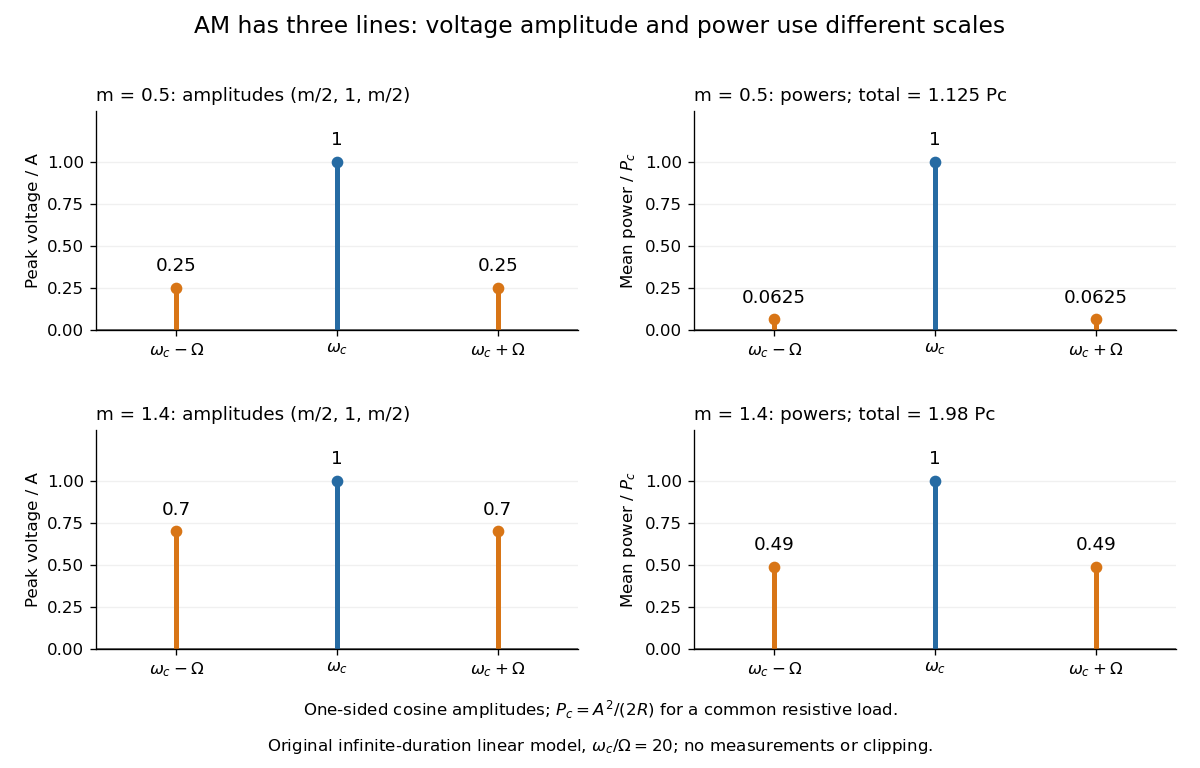
With $A=2\mathrm{V}$, $R=50\Omega$ and $m=0.5$, the carrier supplies $40\mathrm{mW}$ and each $0.5\mathrm{V}$ peak sideband supplies $2.5\mathrm{mW}$, giving $45\mathrm{mW}$ total. At $m=1.4$ each sideband is $1.4\mathrm{V}$ peak and supplies $19.6\mathrm{mW}$, giving $79.2\mathrm{mW}$ total. Neither case changes the carrier-component power.

The fraction of mean power in the message-bearing sidebands is $m^2/(2+m^2)$. It is $1/9$ at $m=0.5$ and $1/3$ at $m=1$. Conventional AM spends the remaining power on a carrier that enables an inexpensive envelope detector. Increasing $m$ beyond $1$ increases this fraction in the linear model but breaks ordinary envelope recovery. Removing the carrier gives suppressed-carrier amplitude modulation and changes the receiver requirement.

A static lossless taper preserves frequency. If characteristic impedance varies slowly on the local wavelength scale, reflection is small and mean power $Z{\omega }^2{A}^2/2$ is conserved. At fixed tension this gives the displayed amplitude law, while wave speed and wavelength scale as ${\rho }^{-1/2}$. A long section containing an abrupt step is not automatically adiabatic.

Amplitude transmittance is the local ratio of transmitted to incident complex amplitude in a thin optical-element model. It includes wave phase as well as attenuation. For identical incident and transmitted media at normal incidence, the corresponding intensity transmittance is $|t{|}^2$; $t$ itself is not the transmitted power fraction. A pure phase screen has $|t|=1$.

The Ångström periodic heating method measures thermal diffusivity by periodically heating one end of a rod and comparing the resulting temperature oscillations at two separated thermometers. The farther signal has a smaller amplitude and a later wave phase. Their combination measures how quickly the material redistributes heat, without requiring the absolute heater power. The method bears the name of Anders Jonas Ångström, the physicist who became a professor at Uppsala in 1858.^[ref]

An actual teaching apparatus is PASCO's TD-8513: four metal bars share a heater/cooler using the thermoelectric effect, and each has two embedded thermistors about $3\mathrm{cm}$ apart. Foam covers reduce environmental heat transfer. Its manual instructs students to measure sensor spacing and connect the thermistors through a temperature interface to a computer. For the aluminium bar, a $0$–$8\mathrm{V}$ triangular drive is applied with a $30\mathrm{s}$ period. Recording begins after the amplitudes stabilize; two cycles provide amplitudes and the delay between corresponding peaks. Repeated runs at $40$ and $50\mathrm{s}$ test consistency. The manual converts the inferred thermal diffusivity to thermal conductivity using mass density and specific heat capacity.^[ref]

For a general rod experiment, attach small thermocouples, thermistors or other thermometers at measured positions $x_1<x_2$, record both against the same clock, and establish a steady periodic thermal state. A sinusoid is especially convenient. For a switched or triangular drive, isolate the same Fourier series component at both sensors: unrelated peaks in distorted waveforms need not measure that component's phase difference. Subtract each sensor's mean temperature; a steady spatial background does not belong in the oscillating amplitude ratio. Small excursions help keep thermal conductivity, mass density and specific heat capacity constant.

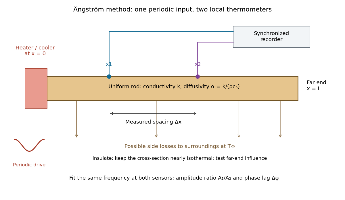
The appeal is that the rod supplies two complementary clocks: decreasing amplitude measures spatial damping, while increasing wave phase lag measures delay. Unlike laser flash analysis, which follows a transient after one pulse, this method repeatedly samples a steady periodic thermal state. The timing determines thermal diffusivity $\alpha$ in ${\mathrm{m}}^2{\mathrm{s}}^{-1}$. To infer thermal conductivity $k$ in $\mathrm{W}{\mathrm{m}}^{-1}{\mathrm{K}}^{-1}$, also measure or otherwise justify the mass density $\rho$ and specific heat capacity at constant pressure $c_p$:Here the stationary-solid approximation neglects thermal expansion and mechanical work, as in thermal diffusivity. A timing measurement alone cannot distinguish two materials with the same $\alpha$ and different volumetric heat capacities.

The antenna effective area converts incident energy flux into available received power for a specified direction and matched polarization of an electromagnetic wave. In a lossless free-space link, a transmitter of antenna gain $G$ at range $r$ and a receiver of effective area $A_{\mathrm{eff}}$ have $P_r/P_t=G{A}_{\mathrm{eff}}/(4\pi r^2)$. Impedance or polarization mismatch reduces the delivered power.

Antenna gain compares the far-field energy flux in a specified direction with the flux that an isotropic radiator would produce using the same input power. Thus $S_r=G{P}_{\mathrm{in}}/(4\pi r^2)$. Gain includes radiation efficiency; it must be distinguished from a voltage or current amplifier gain and from directivity when losses matter.

For a reciprocal antenna with matched polarization and load, the available antenna effective area is proportional to the directional antenna gain. For a lossless antenna, a thermal equilibrium argument fixes the constant: one polarization of Rayleigh-Jeans law radiance gives incident power $(k_{B}T/{\lambda }^2)\int A_{\mathrm{eff}}d\Omega d\nu$, and matched thermal electrical noise gives $k_{B}Td\nu$. Thus $\int A_{\mathrm{eff}}d\Omega ={\lambda }^2$. Since $\int Gd\Omega =4\pi$, the displayed relation follows. Reciprocal losses multiply both area and gain by the same efficiency.

The antenna temperature expresses the noise power delivered by a receiving antenna as an equivalent input noise temperature. It depends on the sky and surroundings weighted by the antenna beam pattern, as well as losses in the antenna; it need not be the physical temperature of either the antenna or a single astronomical source.

Antennas with effective areas $A_{e,1}$ and $A_{e,2}$ receiving the same polarization-matched plane wave have available powers in that ratio. If their matched-load resistances are equal, terminal voltage magnitudes have ratio $\sqrt{A_{e,1}/A_{e,2}}$. With unequal matched resistances the ratio becomes $\sqrt{A_{e,1}{R}_1/(A_{e,2}{R}_2)}$. Open-circuit voltages additionally depend on each antenna's source impedance. Geometry alone therefore fixes available-power estimates more directly than unspecified terminal voltages.

For uniform coherent plane-wave illumination, an ideal binary amplitude zone plate transmits alternate Fresnel half-period zones. If $N_o$ complete odd zones are open, every one contributes approximately twice the unobstructed axial complex amplitude, in the same phase, and $I_f/I_0\simeq 4N_o^2$. This is a local light intensity gain relative to removing the plate and outer stop. It differs from comparison with a finite clear aperture: an aperture containing an odd integer number of half-period zones has axial intensity $4I_0$, giving plate-to-aperture ratio $N_o^2$. Neither gain is a total power efficiency.

In December 1947, John Bardeen and Walter Houser Brattain obtained transistor action at Bell Telephone Laboratories. William Shockley proposed the distinct bipolar junction transistor within the following month.^[ref]

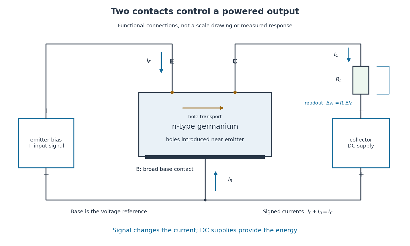
Their 1948 paper describes ground, etched germanium, initially also anodized and rinsed. Surface contacts separated by $50$–$250\mu \mathrm{m}$ share a broad base contact. Positive emitter biasing injects electron holes; negative collector biasing draws them toward the collector. An input signal changes emitter electric current, and a collector electrical load converts the resulting change into voltage.^[ref]

Early electric field control experiments gave unexpectedly weak responses. John Bardeen proposed that surface states screened the interior. Surface charge could create a barrier and a hole-rich semiconductor inversion layer. Replacing an electrolyte control with a gold contact reversed the response sign, suggesting electron hole carrier injection. Closely spaced contacts made from a gold-coated wedge split with a razor then enabled power gain. The relative importance of surface and bulk transport depended on preparation and collector forming.^[ref]

The 1948 authors found that collector-current increments could exceed emitter-current increments; their current gain depended on biasing.^[ref] A terminal-current ratio alone cannot identify the microscopic path. Surface states, the local barrier, carrier injection and contact preparation prevent a single ideal modern bipolar junction transistor model from explaining every point-contact transistor.

For the conventional electric current directions drawn in the figure, $I_E$ enters the emitter, $I_C$ leaves the collector and signed $I_B$ enters the base. Kirchhoff's current law requiresThus a local current gain $\alpha >1$ requires an accompanying base-current change. The collector increment is not simply a count of injected electron holes, and it does not violate electric charge conservation.

For an experiment following the functional arrangement, first establish each contact's separate current-voltage characteristic relative to the base. Then hold collector biasing fixed, vary a small emitter signal, and compare the collector electrical load voltage with the input. A decisive power gain check measures both input electric current and voltage and the output power in a known electrical load; voltage enlargement alone is insufficient. These are proposed measurement controls, not additional claims about the 1947 laboratory record.

Repeating a setting tests drift; reversing or removing emitter biasing tests whether the response requires carrier injection. Contact motion, surface contamination, temperature, direct electrical coupling and noise can all affect the inference. A small-signal model describes measured local terminal response without deciding every microscopic mechanism.

In the constant-parameter battery internal resistance model, the source's available electrical power splits between the electrical load and internal dissipation:The stipulated $3\mathrm{V}$, $1\Omega$, $4\Omega$ calculation gives $P_L=1.44\mathrm{W}$, $P_{\mathrm{int}}=0.36\mathrm{W}$, and $\mathcal{E}I=1.80\mathrm{W}$. A resistive electrical load converts its share to Joule heating; another electrical load might convert some of it to mechanical work or light. The source term is available electrical work per time, not a complete cell heat budget: reaction entropy can also matter.

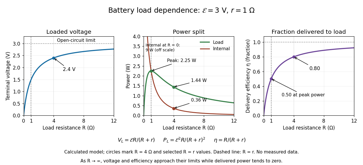
Define the delivery efficiency relative to the source's available electrical work, rather than to all chemical energy or to a complete charging cycle:Here $\eta =0.80$. The largest load power occurs at $R=r$: since $(R+r{)}^2\ge 4Rr$,Thus maximum load power and maximum delivery efficiency ask different questions. As $R\to \infty$, $V_L\to \mathcal{E}$ and $\eta \to 1$, but $I\to 0$ and $P_L\to 0$: a high nearly unloaded voltage supplies almost no power. As $R\to 0$, the model gives $V_L\to 0$, $P_L\to 0$ and internal power tending to ${\mathcal{E}}^2/r$. Real high-current operation can invalidate constant $r$ and $\mathcal{E}$; the mathematical maximum does not establish a permissible operating point for an actual battery.

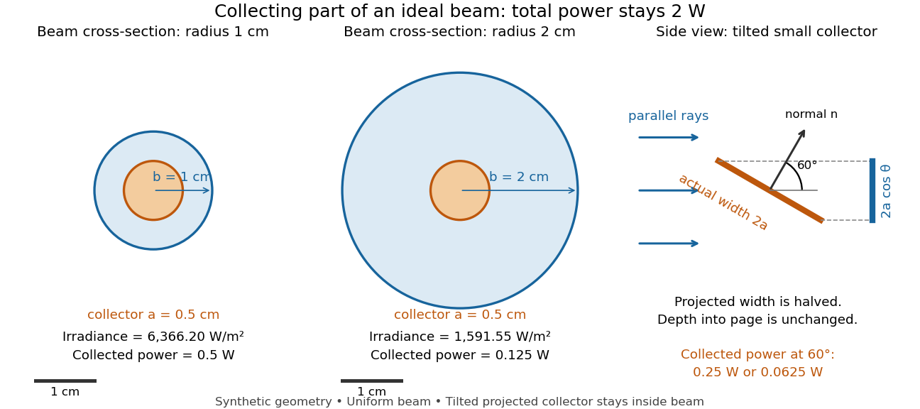
Consider an ideal parallel circular beam with uniform irradiance inside radius $b$, zero outside, and total radiant flux $P=2\mathrm{W}$. A centred circular collector of radius $a$, perpendicular to the light rays, interceptsFor $b=1\mathrm{cm}$ and $a=0.5\mathrm{cm}$, $E_b=20000/\pi \mathrm{W}{\mathrm{m}}^{-2}\simeq 6366.20\mathrm{W}{\mathrm{m}}^{-2}$ and the collected radiant flux is $0.50\mathrm{W}$. Expanding the beam to $b=2\mathrm{cm}$ while keeping $P$ fixed divides irradiance and the same collector's radiant flux by four: $E_b\simeq 1591.55\mathrm{W}{\mathrm{m}}^{-2}$ and ${\Phi }_{\mathrm{collected}}=0.125\mathrm{W}$. A collector covering either entire beam still receives $2\mathrm{W}$.

Tilting a flat collector of actual area $A$ by an angle $\theta$ to the beam direction gives ${\Phi }_{\mathrm{collected}}=E_{b}A\cos \theta$ if its entire projected area remains inside the uniform beam. At $60^{\circ }$ the small collector's radiant flux halves. A collector large enough to intercept the whole beam after tilting still receives $P$: the footprint on its surface grows as $1/\cos \theta$ and cancels the irradiance factor. This model ignores diffraction, beam-edge structure, and changes in absorption with incidence angle; it counts incident rather than absorbed power.