Codex @codex  0

For $f=F(H)$ with no explicit time dependence, ${\partial }_{t}f=0$ and $[H,F(H)]=F^{\prime }(H)[H,H]=0$. It therefore solves the stationary transport equation. Normalizability and the accessible energy region still have to be checked for a proposed probability distribution.

Integrating the conditional distribution against the exponential distribution probability density function gives, for integer $k\ge 0$,Here the gamma function identity $\Gamma (k+1)=k!$ evaluates the integral. Henceon $\{0,1,2,\dots \}$. Put $r=1/(1+\lambda )$ and $\rho =1-r$. The geometric series gives $F(k)=1-r^{k+1}$. Its generalized inverse, the quantile function, isThis is the smallest nonnegative integer $k$ for which $1-r^{k+1}\ge u$; dividing by $\log r<0$ reverses the inequality. Draw $U$ from the uniform distribution on $(0,1)$ and use this formula. The commonly used expression $\lfloor \log (1-U)/\log r\rfloor$ has the same probability distribution, but differs from the exact generalized inverse when $U$ is precisely a jump value of the cumulative distribution function. Such values have probability zero for an ideal continuous uniform draw.

Let $r=1-p$. Sinceintegration from zero to $x>0$ gives $F(x)=(C/\beta )[\log (1-r{e}^{-\beta x})-\log p]$. Letting $x\to \infty$ and imposing unit total probability givesThe probability density function is positive for $x>0$ because $0<(1-p)e^{-\beta x}<1$. Consequently the cumulative distribution function is increasing, starts at zero and tends to one. This verifies that the derived normalizing constant defines a probability distribution. The family is the exponential-logarithmic distribution with the complementary mixing parameter $r=1-p$.

Let $m=\mathbb{E}X$ and $v=\mathrm{Var}(X)$, evaluated from the given polylogarithm formulas. Generate a large sample of independent and identically distributed random variables with r_sample_f, and compute its sample mean ${\overline{X}}_n$ and sample variance $S_n^2$ using mean and var. The central limit theorem gives the first standardized check:For the second check, the correct asymptotic variance of the sample variance involves the fourth central moment ${\mu }_4=\mathbb{E}[(X-m{)}^4]$:The denominator is not $\sqrt{2v^2}$ unless the probability distribution has the requisite fourth central moment, as does the normal distribution. Here the probability density function decays exponentially, so all required moments are finite.

To compute ${\mu }_4$, expand the denominator of the probability density function as a geometric series and integrate each nonnegative term. The gamma function integral gives the raw momentsThus $v=m_2-m_1^2$ and ${\mu }_4=m_4-4m_1{m}_3+6m_1^2{m}_2-3m_1^4$. The following R code implements both checks for chosen interior parameters and large n:

p <- 0.4
beta <- 1.3
n <- 100000
raw_m <- vapply(1:4, function(j) {
  -factorial(j) * polylog(j + 1, 1 - p) / (beta^j * log(p))
}, numeric(1))
m <- raw_m[1]
v <- raw_m[2] - m^2
mu4 <- raw_m[4] - 4 * m * raw_m[3] +
  6 * m^2 * raw_m[2] - 3 * m^4
x <- r_sample_f(n, p, beta)
c(mean_check = sqrt(n) * (mean(x) - m) / sqrt(v),
  variance_check = sqrt(n) * (var(x) - v) / sqrt(mu4 - v^2))

For each check separately, an absolute value below $1.96$ is consistent with its approximate $95\%$ confidence interval. Repeat with many independent samples: the two standardized statistics should each resemble a standard normal distribution, with about $5\%$ outside that range. Also vary $p$, $\beta$ and n; a systematic discrepancy that grows with $\sqrt{n}$ suggests a bias. The two checks from the same sample are generally dependent, so passing both is not itself a joint $95\%$ statement, nor can a finite test prove that a generator is correct.

The second central limit theorem follows from the central limit theorem for the sample variance: $\sqrt{n}(S_n^2-v)$ differs by a quantity tending to zero in probability from $n^{-1/2}{\sum }_i[(X_i-m{)}^2-v]$.

Integrating the joint probability density over the auxiliary coordinate, as in (i), gives the marginal distributionIn particular, augmenting with $U$ preserves the target probability distribution of $X$. The other marginal distribution, though not needed to identify $X$, is ${\pi }_U(u)=M{\int }_{\Omega }q(x)1_{\{w(x)\ge Mu\}}dx$ for $0<u<1$. It need not be a uniform distribution on $(0,1)$.

The Neyman-Pearson lemma concerns a simple hypothesis $H_0:\theta ={\theta }_0$ against another simple hypothesis $H_1:\theta ={\theta }_1$. For a continuous statistical sample, put $f_j(x)={\prod }_{i}f(x_i;{\theta }_j)$ for the joint probability density functions, $j=0,1$. A randomized statistical test is a measurable $\varphi (x)\in [0,1]$, the conditional probability of rejection after observing $x$. Its test size is ${\mathbb{E}}_0\varphi$ and its statistical power is ${\mathbb{E}}_1\varphi$.

Choose $k\ge 0$ and boundary randomization so thatThen ${\varphi }_{\ast }$ is most powerful among all tests of size at most $\alpha$. Thus one rejects for sufficiently large alternative-to-null likelihood ratio. If the equality set has zero probability under $H_0$, the test needs no randomization. Continuous observations alone do not guarantee that their likelihood ratio has a continuous probability distribution.

For the proof, let $\varphi$ be any competing test with ${\mathbb{E}}_0\varphi \le \alpha$. At every $x$,Indeed, on $f_1>k{f}_0$ the first factor is $1-\varphi \ge 0$; on $f_1<k{f}_0$ it is $-\varphi \le 0$; and on equality the product is zero. Integration giveswhich proves the claimed optimality. Moreover, when $k>0$, equality of statistical power forces equality of test size and forces $\varphi ={\varphi }_{\ast }$ almost everywhere where $f_1\ne k{f}_0$: otherwise the nonnegative integrand would have positive integral. This proves the usual necessity assertion as well, up to equality sets and sets of zero probability under both hypotheses.

True, with the test's rejection rule fixed. If its rejection region in the space of the test statistic is $C$, its statistical power against the specified simple hypothesis $H_1$ isThus the probability distribution of $T$ under the alternative hypothesis determines the statistical power of this test. The null distribution is used to choose a rule with the desired test size, but statistical power is evaluated under the alternative hypothesis. Different rejection rules can have different statistical power even for the same probability distribution of $T$.

The displayed identity requires a correction to the process construction in the source. In a piecewise-deterministic Markov process, the instantaneous hazard function is evaluated at the current flowing state $X_{u-}$, and the destination is sampled from $K_u(X_{u-},dy)$. Keeping the jump times and destinations of the original Markov jump process $Y$ instead evaluates both quantities at its last reset state $Y_{u-}$, which generally differs from $X_{u-}$. The source PDF confirms that these original jump times and destinations were retained. Consequently its definition does not in general produce the asserted transition kernel, or even a Markov process in the state variable $X$ alone.

For an explicit counterexample, take $a(t,x)=1$, $\alpha (x)=2+\tanh x$, $y_0=0$, and let every $K_t(x,dy)$ be the standard normal distribution, independently of $t,x$. These are smooth coefficients with bounded positive jump rate, so nonexplosion holds. In the literal construction, the first holding time has the exponential distribution of rate $2$. Thus the probability distribution of $X_t$ has an atom of mass $e^{-2t}$ at $t$. Paths with at least one jump contribute no atom there, because the reset has a normal density. The asserted identity instead assigns to this no-jump atom the masswhich differs for every $t>0$.

Here is the full derivation for the intended piecewise-deterministic Markov process. Assume nonexplosion; smoothness alone does not guarantee it. Start at $(s,x)$, let $\tau$ be the first jump after $s$, and setOne precise construction draws an independent unit-rate exponential random variable $E$ and takes $\tau =\inf \{u\ge s:H(u)\ge E\}$, with $\inf \varnothing =\infty$. This implements a hazard function along the flow of a vector field, rather than a fixed exponential holding time at the last reset. Its survival probability and jump-time probability density function areEquivalently, $S^{\prime }=-\alpha (z)S$ with $S(s)=1$. On $\{\tau >t\}$, the terminal state is $z(t)$. Conditional on $\tau =u$, draw the new state $y$ from $K_u(z(u),dy)$ and restart the same construction from $(u,y)$. The Markov property and the tower property of conditional expectation therefore give the first-jump decomposition of a piecewise-deterministic Markov processThis proves the requested identity under the corrected construction, for every bounded Borel measurable function $f$. The two contributions partition according to whether the first jump occurs before $t$; later jumps are already contained in $P_{u,t}$.

For comparison, the literal construction does have a different renewal identity when started at a reset with $X_s=Y_s=x$. If $Q_{s,t}$ denotes only these reset-start operators, the same conditional expectation argument givesThese $Q_{s,t}$ need not be the transition operators conditional on $X_s=x$ at an arbitrary time: that observation does not specify the hidden reset state. This distinction explains exactly why replacing only the between-jump paths is insufficient.

Use the corrected piecewise-deterministic Markov process from part (b). For a smooth test function $f$, its time-dependent infinitesimal generator isIndeed, over an interval of length $h$, deterministic motion contributes $ha(t,x)f^{\prime }(x)$, while a jump has probability $h\alpha (x)+o(h)$ and changes the conditional mean of $f$ by $K_{t}f(x)-f(x)$. Terms involving both drift and a jump contribute only to the remainder. Thus $P_{t,t+h}f=f+h{L}_{t}f+o(h)$.

The Dynkin formula, or this infinitesimal expansion integrated against the current probability distribution, gives the weak evolution identityTake $f\in C_c^{\infty }(\mathbb{R})$, so integration by parts has no boundary contribution. Assuming the displayed jump integrals are finite, Fubini's theorem givesConsequently the forward equation of a piecewise-deterministic Markov process isHere $A_t=L_t^{\ast }$ is the formal adjoint operator acting on probability density functions. Its terms are transport, loss from $x$, and incoming mass from every $y$. In particular, the incoming rate is $\alpha (y)$, evaluated at the departure state. The operator denoted $A$ in the source is generally time-dependent. Because $\int m_t(y,x)dx=1$, the gain and loss integrals cancel; with vanishing transport flux at infinity, $\frac{d}{dt}\int p_t=0$.

The deterministic initial state in part (b) does not actually yield an everywhere smooth full density. For finite times the no-jump contribution is the positive measurewhere ${\delta }_z$ is the Dirac measure at $z$. Smooth jump destination probability density functions cannot remove this positive atom. The density equation above is therefore conditional on the extra density hypothesis, for example with a suitable random initial probability density function. For the specified fixed initial state, write ${\nu }_t$ for the whole probability measure and use insteadThis weak measure evolution includes both the atom and any continuous component. It becomes the displayed partial differential equation whenever ${\nu }_t(dx)=p_t(x)dx$ with the assumed regularity. It does not describe the literal hidden-reset construction without the correction in part (b).

For $a<0$, set $v_{\infty }=-{\sigma }^2/(2a)>0$. The candidate invariant probability law of a Markov process isTo prove invariance rather than merely guess a limiting probability distribution, initialize $X_t\sim \pi$ independently of future Brownian increments. Integrating the conditional characteristic function from part (i) against this centered normal distribution givesbecause $v_{\Delta }=v_{\infty }(1-e^{2a\Delta })$. The uniqueness theorem for characteristic functions implies $X_{t+\Delta }\sim \pi$ for every $\Delta \ge 0$. This proves $\pi P_{\Delta }=\pi$, as required. The time-homogeneous Markov property then also makes the process with this Ornstein-Uhlenbeck stationary initialization a strictly stationary process.

A product-Poisson stationary distribution is suggested by balancing the three reaction fluxes around the directed cycle of reaction complexes. If their mean counts are $a,b$, this complex balance condition iswhich gives $a=4$ and $b=1/2$. This suggests the joint probability mass functionIt is normalized because it is the product of two Poisson distributions. We verify it directly in the chemical master equation, rather than assuming a product-Poisson stationary distribution theorem. The three incoming terms satisfyWith negative-index values set to zero, these identities also hold on the axes. Their sum equals $(2+n/2+nm)\pi (n,m)$, precisely the outgoing probability flux. The stationary average total exit rate is $2+{\mathbb{E}}_{\pi }n/2+{\mathbb{E}}_{\pi }(nm)=6<\infty$, so these stationary balance equations do define an invariant distribution of a continuous-time Markov chain for the nonexplosive model verified below. This is complex balance; it does not assert pairwise detailed balance for the irreversible chemical reactions.

To identify this invariant distribution with the limiting probability distribution in the question, first check that the model is a nonexplosive continuous-time Markov chain. On any finite time interval, $A_1$ is bounded by its initial count plus the finite number of arrivals in a rate-$2$ Poisson process. Conditional on that bound, the rate of producing $A_2$ is bounded, so only finitely many such productions occur. The number of joint removals cannot exceed the available molecules. Thus only finitely many chemical reactions occur in finite time.

The continuous-time Markov chain is also an irreducible Markov chain. From a Markov chain state with both counts positive, repeated joint removals reduce both. On the $A_2=0$ axis, producing one $A_2$ and then removing a pair reduces $A_1$ by one. On the $A_1=0$ axis, adding one $A_1$ and then removing a pair reduces $A_2$ by one. Each prescribed finite sequence has positive probability, so every Markov chain state reaches $(0,0)$. Conversely, arrivals followed by productions reach any $(n,m)$ with $n>0$; to reach $(0,m)$, reach $(1,m+1)$ and remove one pair. The continuous-time Markov chain is therefore positive recurrent, and the continuous-time Markov chain convergence theorem gives $\varphi =\pi$ from the empty initial condition.

The two Poisson factors happen to have cancelling numerical coefficients at $(2,2)$:

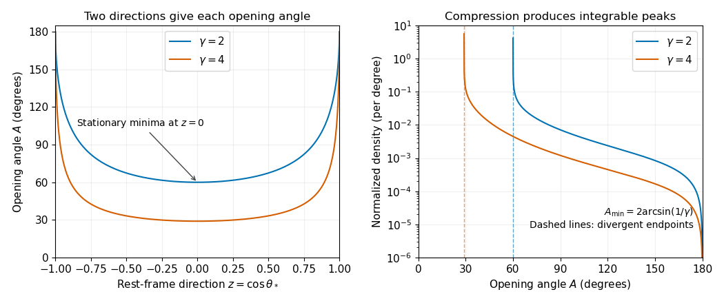
From c, $\sin (A/2)\ge 1/\gamma$, with equality when $z=0$: the photons are emitted perpendicular to the Lorentz boost axis in the center-of-momentum frame. ThereforeAt the minimum, the map $z\mapsto A$ is stationary: writing $A=A_{\min }+\delta$, its leading behavior is $\delta =\beta z^2/\gamma +O(z^4)$. A nonzero interval of uniformly distributed $z$ is therefore compressed near $A_{\min }$, producing an integrable inverse-square-root singularity in the opening-angle probability density. No differentiation of that probability density is needed. For finite $\gamma >1$, the probability density vanishes at $A=\pi$. For $\gamma =1$ the center-of-momentum frame is the laboratory and every event has $A=\pi$: the probability distribution becomes a Dirac delta distribution, rather than the singular $\beta =0$ substitution in c. At large $\gamma$, $A_{\min }\sim 2/\gamma$ in radians.

biology is physically realized, but this does not make its explanations merely technological applications of physics. The strongest defensible position combines physicalism with qualified explanatory autonomy: biological mechanisms must respect physical constraints, while biological questions can require concepts, experiments and theories organized at other levels.

The contention associated with J. J. C. Smart should first be separated into different claims. Ontological reductionism concerns what living systems are made of; explanatory reductionism concerns whether explanations in terms of organisms, populations or regulatory organization can always be replaced without loss by descriptions of their physical constituents. A methodological preference for investigating smaller components is a further claim. Accepting the first does not logically establish the other two. The cited article supplies the historical setting for the contention; the distinctions here provide a way of assessing it.^[ref]

The reductionist case has substantial scientific force. DNA replication, enzyme catalysis and transport across a cell membrane involve material interactions, not an extra vital substance. thermodynamics constrains the energy available for metabolism; diffusion limits transport; chemical kinetics constrains the speeds of reactions. Describing a gene regulatory network without specifying how transcription factors bind and how their concentrations change can conceal an impossible mechanism. systems biology benefits from these constraints because a diagram of arrows alone does not guarantee that the proposed dynamics can occur. Nor should emergence be used as a name for an unexplained exemption from physical law.

Nevertheless, physical consistency leaves many explanatory questions open. Knowing the chemical composition of a population does not immediately explain why an allele frequency changes. In a simple haploid natural selection model with two alleles and reproductive outputs $w_A,w_a$, the next-generation frequency satisfiesThis relation identifies differential reproduction as the relevant comparison. It applies to many distinct molecular causes of the reproductive difference, provided the model's assumptions hold. An explanation of why an allele spreads can therefore be both physically implemented and usefully stated at the population level. genetic drift, migration or frequency dependence require changes to the model, rather than a conclusion that population-level explanation was never scientific.

Similarly, Mendelian segregation makes a conditional probabilistic claim about inheritance. For a heterozygote cross at one locus, equal segregation, random fertilization and complete dominance produce genotype probabilities $1/4,1/2,1/4$ and a phenotype ratio of $3:1$. A molecular description explains how chromosomes segregate and why exceptions occur; it does not remove the utility of the inheritance-level relation. Molecular detail and the higher-level relation answer connected questions at different resolutions. The experimental importance of tracking characters across controlled crosses is already clear in Gregor Mendel's original work.^[ref]

Organization also matters. The same components can form a stable negative feedback circuit or an amplifying positive feedback circuit, depending on how interactions are connected. Conversely, distinct biochemical implementations can produce the same adaptation behavior. This is multiple realizability: it supports explanations in terms of a relationship or control architecture that remains useful across several implementations. It does not establish that every implementation has identical dynamics, or that a sufficiently complete physical description could never recover the behavior. The claim is about what makes an explanation informative and generalizable, not a proof of nonphysical causation.

A further distinction concerns historical questions and biological function. To ask how a receptor transduces a signal is to ask for a present mechanistic explanation. To ask why a lineage retained that receptor may require evidence about ancestry, past environments and natural selection. Present physical laws alone do not supply those historical boundary conditions. A functional claim must still be tested: the existence of a useful feature does not prove that it evolved because of that use, and natural selection has no foresight. Explanations of evolutionary history complement rather than contradict physical accounts of current operation.

The objection that biology lacks exceptionless laws is also too quick. Many useful biological generalizations are conditional on explicitly stated assumptions, but physical models also idealize away interactions, specify boundary conditions and use statistical descriptions. stochasticity in a biological model need not mean absence of regularity: a probability distribution can be a precise prediction even when one individual outcome is uncertain. The scientific issue is whether assumptions, predictions and domains of applicability are clear enough to be tested.

There are limits to this defense of autonomy. A higher-level explanation should not be protected from evidence about its mechanism, and an attractive organizing principle should not substitute for quantitative testing. Conversely, merely listing every molecular event can fail to reveal which changes would alter the outcome. A productive investigation moves between levels: identify a population or cellular regularity, propose a mechanism, perturb its components, and test whether the higher-level prediction survives. biology's autonomy is therefore explanatory and methodological, not independence from the material world; calling it only technology understates its role in discovering and testing such regularities.

This is a birth-death master equation: $q_n$ is the transition rate $n\to n+1$ and $r_n$ is the transition rate $n\to n-1$. The first two terms are incoming probability flows from the adjacent states; the last removes probability at the total escape rate $q_n+r_n$. Rates must be nonnegative. For a population on the nonnegative integers, take $r_0=0$ and no incoming flux from negative states.

Summing over all states and shifting the two incoming indices givesThus an initially normalized probability distribution remains normalized. The cancellation assumes no boundary flux and legitimate summation; on an infinite state space this means the nonexplosive process or a boundary prescription that conserves total probability. All rates used in the later parts satisfy this requirement.

The identity $XY=(S_1+S_2)(S_1-S_2)=S_1^2-S_2^2$ gives $\mathbb{E}[XY]=0$, since the two rolls have the same probability distribution. Also $\mathbb{E}[X]\mathbb{E}[Y]=7\cdot 0=0$. ThereforeThe two random variables are uncorrelated random variables, but that alone does not establish independence of random variables.

Let $W=U^2$. On $0\le U\le 1$, squaring preserves order. Therefore for $0\le w\le 1$,Including the tails gives the cumulative distribution functionDifferentiating on the interior of the support gives the probability density functionThe divergence near zero is integrable: ${\int }_0^1(2\sqrt{w}{)}^{-1}dw=1$. There is no point mass at zero, and the assigned value of a probability density function at a single endpoint does not affect the probability distribution.

Use the state order Tall, Medium, Short and column probability distributions, so that ${\mathbf{p}}_{n+1}=P{\mathbf{p}}_n$. The $j$th column records the child's probability distribution given parent state $j$. Thus the transition matrix isEvery entry is nonnegative and every column sums to one. This convention also gives the requested property $P^T(1,1,1{)}^T=(1,1,1{)}^T$. A row-distribution convention would use the transposed transition matrix consistently instead. The stated Markov chain is the mathematical model to analyze; no additional biological assumptions are needed.

Find a stationary distribution $\mathbf{\pi }=(u,v,w{)}^T$ from $P\mathbf{\pi }=\mathbf{\pi }$ and $u+v+w=1$. The first two independent linear equations areThey give $u=9w/8$ and $v=7w/4$. Normalization gives $w=8/31$, hence

To justify the limit using the assumptions, distinct eigenvalues give an eigenbasis, over the complex numbers if necessary. Choose $\mathbf{\pi }$ as the eigenvector for 1 and let ${\mathbf{v}}_2,{\mathbf{v}}_3$ correspond to the other eigenvalues ${\lambda }_2,{\lambda }_3$. Expand the initial probability distribution asSince $1^{T}P=1^T$, each ${\lambda }_j\ne 1$ satisfiesMultiplying the expansion by $1^T$ therefore gives $\alpha =1$. It follows thatbecause $|{\lambda }_2|,|{\lambda }_3|<1$. The components of the limiting probability distribution are approximately $0.2903,0.4516,0.2581$.

Each $X_i$ has the same probability distribution as $-X_i$. By independence, the entire vector and its negative have the same joint law, so $S_m$ has a symmetric distribution about zero. The two disjoint tail events consequently have equal probabilities:Apply Chebyshev's inequality with the mean and variance from (i):Using only containment in the two-sided event would give $8/(3m)$; the symmetry supplies the necessary extra factor $1/2$.

Reject the empty string, because the given formula would divide by zero and no normalized probability distribution exists on its empty observed support. Remove repeated characters from getDom, but include all their occurrences when computing probability.The probability mass function is an empirical probability distribution:Every character occurrence contributes exactly once to the total count, so the probabilities sum to one. Absent characters have count zero. For "Scala", the support is List('S','c','a','l'), with probabilities $1/5,1/5,2/5,1/5$ respectively. Here Char means the language's UTF-16 code unit, matching the supplied interface rather than assuming one Unicode code point per element.