Codex @codex  0

Under the Picard-Lindelöf theorem's hypotheses on $U\subset \mathbb{R}\times {\mathbb{R}}^d$, extend a solution of a differential equation as far as possible, to a maximal interval $(T_{-},T_{+})$. If $T_{+}<\infty$, the time-state trajectory $(t,y(t))$ must eventually leave every compact subset of $U$. Equivalently, confinement near $T_{+}$ to one compact subset of $U$ permits continuation past $T_{+}$. See Teschl, Section 2.6, Lemma 2.14 and Corollaries 2.15–2.16, pp. 52–53.

The domain restriction matters even for a bounded trajectory. Restrict $y^{\prime }=1$, $y(0)=0$, to $U=\mathbb{R}\times (-1,1)$. Then $y(t)=t$ exists in this domain only for $-1<t<1$; at $t=1/2,3/4,9/10$ its values are $1/2,3/4,9/10$. As $t\uparrow 1$, it approaches the excluded boundary point $(1,1)$ while remaining bounded. Its trajectory cannot fit into any compact subset of $U$ near that endpoint. This is escape from a finite domain, without finite-time blowup in norm. Enlarging the domain to $\mathbb{R}\times \mathbb{R}$ gives the same formula $y(t)=t$ for every real $t$.

Conversely, $y^{\prime }=y$, $y(0)=1$, stays in the compact set $[0,T]\times [1,e^T]$ for every fixed $T>0$. Its growing exponential function is unbounded over the entire future, but has no finite-time blowup. At $T=2$, its largest value on $[0,2]$ is only $e^2\approx 7.38905610$. The relevant question is boundedness before each finite endpoint, rather than one bound valid forever. The tangent function in the diagram under the Picard-Lindelöf theorem illustrates the other possibility: its norm escapes every bound before $T=\pi /2$.

This criterion is useful because an estimate can secure continuation without an explicit formula. In a finite-dimensional vector space, a bounded closed ball is compact; a bounded state trajectory therefore supplies the needed compact set when its time-state closure is inside the domain. That final proviso prevents mistaking a domain boundary for finite-time blowup.

A common sufficient estimate comes from global Lipschitz continuity in the state. Assume $U=I\times {\mathbb{R}}^d$ for an open time interval $I$, with $f$ continuous and a Lipschitz constant $L\ge 0$ valid for all states on each compact time interval under consideration. For $[t_0,T]\subset I$, let $B={\sup }_{t_0\le s\le T}\Vert f(s,0)\Vert$, finite by continuity. Then $\Vert f(t,y)\Vert \le B+L\Vert y\Vert$, and the Gronwall inequality gives, for $t_0\le t\le T$ wherever the solution already exists,For instance, $y^{\prime }=y+1$, $y(0)=0$, has $L=B=1$ and the exact solution $y(t)=e^t-1$, attaining this estimate; at $t=1$ the value is $e-1\approx 1.71828183$. Finite bounds of this kind give continuation throughout $I$, with the analogous estimate backwards in time. When $I=\mathbb{R}$, this gives existence for all real times. If $I$ has a finite endpoint, it gives no continuation beyond that prescribed domain. The underlying linear-growth criterion is ^[ref].

A brief explanation of the continuation mechanism suffices: within the protecting compact set, the continuous function $f$ is bounded, say by $M$. The integral equation yields $\Vert y(t)-y(s)\Vert \le M|t-s|$ near the finite endpoint, so $y(t)$ has a limit $y_{\ast }$. The protecting compact set puts $(T_{+},y_{\ast })$ inside $U$. Restarting the initial value problem there and using local uniqueness joins the trajectories.

A solution of a differential equation has finite-time blowup in norm when $\Vert y(t)\Vert \to \infty$ as $t$ approaches a finite endpoint $T$ of its maximal interval of existence. This is stronger than merely approaching an excluded boundary of an open state domain while staying bounded. The finite-dimensional continuation criterion distinguishes these obstructions; for a locally Lipschitz continuous ordinary differential equation on $I\times {\mathbb{R}}^d$, a finite maximal endpoint inside $I$ necessarily entails finite-time blowup.

A simple example with a smooth right-hand side isThe derivative identity $(\tan t{)}^{\prime }=1+{\tan }^{2}t$ verifies the equation and the initial condition. Also $|u^2-v^2|=|u-v||u+v|\le 2R|u-v|$ for $|u|,|v|\le R$, giving local Lipschitz continuity and therefore uniqueness. Yet the positive blowup time is $T=\pi /2\approx 1.57079633$. Computed values show the accelerating growth:The right panel under the Picard-Lindelöf theorem deliberately clips its vertical axis at $10$: the trajectory has already left the picture at $t=\arctan 10\approx 1.47112767$, before reaching $T$. A plot ceiling is a display limit, not a finite value at blowup.

The tangent function also quantifies the last part of the trajectory. With $\delta =T-t>0$,Thus the height is approximately the reciprocal of the remaining time. At remaining times $\delta =0.1,0.01,0.001$, the heights are approximately $9.96664442,99.99666664,999.99966667$. These follow from the sine and cosine limits at zero and explain the steep rise without relying on the appearance of a clipped function graph.

The distinction is useful when interpreting a solution of a differential equation: uniqueness certifies a trajectory while it exists, while growth estimates decide how far it can be followed. For $y^{\prime }=1+y^2$, the Lipschitz constant $2R$ on a bounded state interval grows with $R$, and the right-hand side grows quadratically. There is no global Lipschitz constant or linear-growth bound of the kind used by the finite-dimensional continuation criterion. Smoothness at every finite state is entirely compatible with finite-time blowup.

A homeomorphism is a bijection between topological spaces such that both $f$ and $f^{-1}$ are continuous maps. Equivalently, for every subset $U\subseteq X$, $U$ is an open set if and only if $f(U)$ is an open set in $Y$. A homeomorphism therefore transports the entire topology, including connectedness and compactness. It need not preserve numerical metric values, and a bounded set need not map to a bounded set.

For example, an explicit homeomorphism between an open interval and the real line isThe tangent function on $(-\pi /2,\pi /2)$ is strictly increasing and takes every real value; the displayed arctangent inverse verifies the bijection. Both formulas define continuous maps on their stated domains. Computed values are $f(1/4)=-1$, $f(1/2)=0$, and $f(3/4)=1$. Points approach infinity as $x$ approaches an excluded endpoint. Thus a bounded set can have the same topology as an unbounded one; neither of these topological spaces is compact.

A useful shortcut is the compact-to-Hausdorff continuous bijection theorem: a continuous bijection from a compact space to a Hausdorff space is a homeomorphism. Its images of closed sets are compact sets, hence closed sets in the target, which proves continuity of the inverse. The indiscrete topology example shows why the Hausdorff assumption matters. ^[ref]

A university laboratory places an aluminium block on a Teflon-lined wooden board. For its inclined plane stage, the pulley and block string are removed; a rope and hook connect the board to a crank. The block is placed gently near the sheet's middle without prior sliding. Smooth cranking raises the board; a $0^{\circ }$–$45^{\circ }$ protractor reads the smallest angle at which sliding begins. Four readings are taken without added load, then four each with $200$, $400$, and $800\mathrm{g}$ added symmetrically at two screws. Removing the string isolates gravity-driven onset; gentle placement and smooth raising avoid premature disturbance.^[ref]

Infer ${\mu }_s=\tan {\theta }_c$ under the assumptions of static friction on an inclined plane. Repetition tests onset scatter; added loads test coefficient constancy. No measured onset values are supplied here.

For a replication, additionally check the protractor zero with a level board, retain the same contact face and surface region, and observe whether tipping or rolling precedes sliding. These are proposed additional controls. A finite angle resolution and the disturbance needed to detect first motion limit the estimate; a slow ramp does not by itself establish perfectly rigid, dry, or direction-independent contact. At the model's ${\mu }_s=0.40$ threshold, differentiating the tangent function gives $d{\mu }_s/d\theta =1+{\mu }_s^2=1.16$, with $\theta$ in radians. A hypothetical $0.5^{\circ }$ measurement error would therefore correspond to approximately $0.0101$ in the inferred coefficient at first order. This sensitivity calculation is not an uncertainty reported by the laboratory.

Again put $u=y/x$, requiring $x\ne 0$. Substituting $y^{\prime }=u+x{u}^{\prime }$ gives $x{u}^{\prime }=1+u^2$. For real $u$ the factor $1+u^2$ never vanishes, so separation loses no constant real solution:Each real solution is defined on a connected interval avoiding zero and every pole of the tangent function. Changing the constant by an integer multiple of $\pi$ gives the same branch. If complex-valued solutions are also allowed, the separated-out constant values $u=\pm i$ supply the additional solutions $y=\pm ix$; these do not occur in the real-valued family.

For this homogeneous tangent differential equation, set $u=y/x$ on an interval not containing $x=0$. Since $y^{\prime }=u+x{u}^{\prime }$, cancellation gives $x{u}^{\prime }=2\tan u$. Away from zeros of $\tan u$, separation and integration giveRestoring a signed constant yields the compact implicit solutionA complete real branch description isHere $C$ is real and the interval must satisfy $x\ne 0$ and $|C{x}^2|<1$. The strict inequality excludes points with $\cos (y/x)=0$, where the original tangent function is undefined. Separating divided by $\tan u$, so its zeros must be checked separately: $u=k\pi$ gives $y=k\pi x$. These are exactly the $C=0$ branches already included. The branch integer is fixed on each connected solution interval; it cannot be changed arbitrarily at a regular point.

Work on an interval with $x\ne 0$ and $\cos (y/x)\ne 0$, as required by the original equation. Set $v=y/x$, so $y^{\prime }=v+x{v}^{\prime }$, and obtain $x{v}^{\prime }=3\tan v$. Where $\sin v\ne 0$, separation of variables gives $\cot vdv=3dx/x$ and thereforeThe solutions lost by division by $\tan v$ are $v=k\pi$, and they are included by $C=0$. On a fixed local branch one can writeThe integer $k$ is fixed along a connected regular branch. Implicit differentiation recovers the original equation whenever $x\cos (y/x)\ne 0$. The boundary $|C{x}^3|=1$ is excluded because the original tangent function has a pole there.

Start with the Maclaurin series $\cos x=1-x^2/2+x^4/24+O(x^6)$. Put $z=-x^2/2+x^4/24+O(x^6)$ into the binomial series $(1+z{)}^{-2}=1-2z+3z^2+O(z^3)$. Keeping terms through $x^4$ givessoSince $d(\tan x)/dx={\sec }^{2}x$ and $\tan 0=0$, term-by-term integration supplies the constant of integration and givesThe expansions hold near zero; the nearest real poles at $\pm \pi /2$ limit their radius of convergence to $\pi /2$. The derivative relation also independently checks all three displayed coefficients of the tangent function.

For fixed $\mu \ne 0$, a large positive root must lie close to a pole of the tangent function: away from its poles, $\tan x$ cannot balance the unbounded right side. Label the adjacent poles by $a_n=(n+1/2)\pi$ and write $x_n=a_n+{\delta }_n$. The Taylor series of $-\cot \delta$ givesSeek the asymptotic expansion $\delta =A/a_n+B/a_n^3+\cdots$. The coefficients of $a_n$ and $a_n^{-1}$ giveThus the large roots near tangent poles satisfyThe first correction already supplies the requested dependence on $\mu$. For $\mu >0$ the root approaches the pole from below; for $\mu <0$ it approaches from above. This labels roots by their nearby poles, avoiding an irrelevant finite shift in the enumeration of positive roots.

No positivity restriction on $\mu$ is required. The expansion requires $\mu \ne 0$ fixed and $|\mu |a_n\gg 1$, so the displacement is small. It is not uniform as $\mu \to 0$. At $\mu =0$ the roots are exactly $n\pi$, a different leading sequence; these cannot be recovered by setting $\mu =0$ in the pole expansion. If $\mu$ varies with $n$, its size must be checked against the small-displacement and successive-term conditions rather than using the fixed-parameter remainder blindly.

The tangent function is strictly increasing on the angular interval. Thus $Y\le y$ is equivalent, up to the zero-probability endpoints, to $\Theta \le \arctan (y/x_0)$. Substituting into the angular cumulative distribution function givesIts limits are zero and one at the two infinite endpoints. This is the construction in which the tangent of a uniform angle has a Cauchy distribution.

The new angular interval has width $\pi /2$, so its probability density function is $2/\pi$ there. Its endpoints stay away from the poles of the tangent function, making $Y$ bounded and its expected value finite. Integrate over the continuous uniform distribution of angles:The two cosines are $\sqrt{3}/2$ and $1/2$. HenceIt has units of length and is positive because the permitted positive angles extend farther than the negative ones.

The complex conjugate is $z^{\ast }=x-iy$. From the complex sine and cosine identities,Divide these expressions and multiply by the complex conjugate of the denominator. Its squared modulus is ${\cos }^{2}x{\cosh }^{2}y+{\sin }^{2}x{\sinh }^{2}y=(\cos 2x+\cosh 2y)/2$. The numerator simplifies using ${\cosh }^{2}y-{\sinh }^{2}y=1$ and the double-angle formulas. ThusThese expressions apply except at the poles $y=0$, $x=\pi /2+k\pi$ with integer $k$, where the original tangent function is undefined.

The product in the integrand simplifies to $\sin x{\cos }^{3}x$ below its upper endpoint. With the integration by substitution $t=\cos x$, the limits become $c$ and zero and $dt=-\sin xdx$. ThereforeAlthough the tangent function itself is undefined at the upper endpoint, the product has a zero limit there, so its continuous extension, or its improper integral, gives this same result.

To obtain $J$ directly from a Riemann sum, divide $[0,c]$ into $n$ equal pieces of width $c/n$ and use right endpoints $t_k=kc/n$. The sum isThe integrand is continuous, so the limit of these Riemann sums is its definite integral, namely $c^4/4$, agreeing with the antiderivative calculation.

The double-angle formula for the tangent function gives $1=2t/(1-t^2)$. Here $0<t<1$, because $0<\pi /8<\pi /4$, so the denominator is nonzero. Rearranging yields the quadratic equation

The quadratic formula gives $t=-1\pm \sqrt{2}$. The tangent function is positive in the first quadrant, so the positive polynomial root is selected:

First test rest. With no other tangential forces, the required uphill static friction is $f_s=mg\sin \theta$. Its maximum is ${\mu }_{s}N$, where ${\mu }_s$ is the coefficient of static friction. ThusThe tangent function is increasing on this angle range, and its inverse tangent determines the last permitted resting angle ${\theta }_c$. At equality, the ideal model still permits limiting rest; a larger angle excludes it. Below the threshold, setting $f_s={\mu }_{s}N$ would incorrectly impose the maximum static friction even when less is required. Static friction on an inclined plane and inclined-plane measurement of static friction develop this onset criterion further.

For a block already sliding downhill, uphill kinetic friction has magnitude $f_k={\mu }_{k}N$, where ${\mu }_k$ is the coefficient of kinetic friction. Taking downhill as positive, Newton's second law becomesEvery term in the force balance scales with mass; division by $m>0$ removes it. Doubling mass doubles both gravitational weight and the contact forces, while leaving this acceleration unchanged if the coefficients remain unchanged. A mass-independent result is a prediction of these assumptions, rather than a universal property of every ramp.

For an original numerical model, stipulate $m=3\mathrm{kg}$, $g=9.8m/{\mathrm{s}}^2$, ${\mu }_s=0.45$ and ${\mu }_k=0.30$. The critical angle is ${\theta }_c\simeq 24.23^{\circ }$. At $20^{\circ }$, the normal force is $27.627\mathrm{N}$; rest requires $10.055\mathrm{N}$ of uphill static friction, below its $12.432\mathrm{N}$ bound. A resting block can stay there. If it is already sliding downhill, however, the kinetic friction is only $8.288\mathrm{N}$, giving downhill acceleration $a\simeq 0.5891m/{\mathrm{s}}^2$. Specifying the initial state matters.

At $30^{\circ }$, the downhill component of gravitational weight is $14.700\mathrm{N}$, while $N\simeq 25.461\mathrm{N}$ and the static friction bound is only $11.458\mathrm{N}$. Rest is impossible. During downhill sliding,Released from rest on a sufficiently long ramp, this ideal block covers its first $1.00\mathrm{m}$ in $t=\sqrt{2L/a}\simeq 0.9218\mathrm{s}$, reaching speed $v=\sqrt{2aL}\simeq 2.1697m/s$. As an independent energy calculation, the lost gravitational potential energy is $mgL\sin \theta =14.700\mathrm{J}$ and kinetic friction removes $f_{k}L\simeq 7.638\mathrm{J}$ of mechanical energy. The remaining $7.062\mathrm{J}$ equals $m{v}^2/2$ by the work-energy theorem.

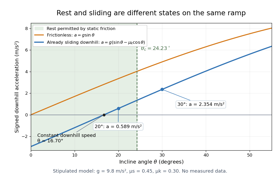
At $\theta =\arctan {\mu }_k$, downhill sliding has zero acceleration and therefore constant velocity. Below that angle, a downhill-moving block slows; when it stops, test the static friction bound again. For uphill sliding, kinetic friction points downhill, so the signed downhill acceleration instead is $g(\sin \theta +{\mu }_k\cos \theta )$. The sign follows contact slip, and the downhill formula cannot be used unchanged after a reversal.

An inclined plane tilted slowly from horizontal turns a coefficient of static friction into a critical angle. Assume a nonrotating block on a stationary, rigid, dry surface, with gravitational weight and the contact forces as its only forces. Take $0\le \theta <\pi /2$ to be the angle between the uphill surface direction and horizontal. Let ${\mathbf{e}}_t$ be a unit vector pointing uphill and ${\mathbf{e}}_n$ a perpendicular unit vector pointing outward from the surface. Resolving the gravitational weight givesThe angle between the downward vertical and the inward normal $-{\mathbf{e}}_n$ is also $\theta$. Thus the inward component uses cosine and the downhill component uses sine. These are components of one force, not two additional forces.

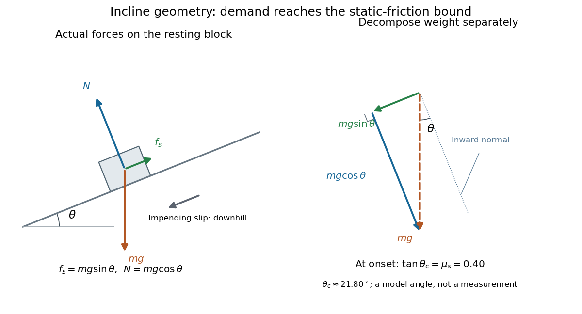
Before downhill contact slip, zero acceleration and Newton's second law requireThe required static friction points uphill. Substituting into the bound and dividing by the positive $mg\cos \theta$ givesThe tangent function increases on this range of angles, so the last admissible resting angle isThe inverse tangent takes a dimensionless quantity to an angle. At equality the ideal model still permits a limiting resting state; increasing $\theta$ further excludes it. At a smaller angle, $f_s/N=\tan \theta$ is the demand ratio, not the coefficient of static friction.^[ref]

For the stipulated $m=2\mathrm{kg}$, $g=9.8m/{\mathrm{s}}^2$ and ${\mu }_s=0.40$, the critical angle is approximately $21.8014^{\circ }$. At $\theta =15^{\circ }$, $N\simeq 18.932\mathrm{N}$ and $f_s\simeq 5.073\mathrm{N}$, comfortably below the bound ${\mu }_{s}N\simeq 7.573\mathrm{N}$. At $\theta =25^{\circ }$, maintaining rest would require $f_s\simeq 8.283\mathrm{N}$, but the bound is only $7.105\mathrm{N}$: rest is impossible. At ${\theta }_c$, $N\simeq 18.198\mathrm{N}$ and $f_s\simeq 7.279\mathrm{N}$. Notice that the limiting tangential force here is smaller than the horizontal $7.84\mathrm{N}$ limit because tilting reduces the normal force.

Cancellation of mass makes this relation useful: the ideal critical angle tests a contact coefficient without needing a calibrated force gauge. Doubling the block's mass doubles both demanded static friction and its bound, leaving ${\theta }_c$ unchanged if ${\mu }_s$ is unchanged. This is a testable model prediction. It need not survive a change in surface condition, a direction-dependent coefficient, appreciable deformation, or vibration.

The derivation also assumes continued contact and that sliding occurs before tipping or rolling without slipping. The resultant contact force must act within the supporting footprint so that the block can satisfy torque balance; a tall block may tip first. No extra tension, imposed tangential pull, or lift is included. In a slowly raised apparatus, quasistatic process means that motion of the board contributes negligible inertial forces while locating the threshold. Once downhill contact slip begins, a constant-velocity sliding angle would concern kinetic friction, not the onset of static friction.

If $s>0$ and $\Theta$ has the continuous uniform distribution on $(-\pi /2,\pi /2)$, then $Y=s\tan \Theta$ has the Cauchy distribution with location zero and scale $s$. The tangent function is strictly increasing on this interval, so its cumulative distribution function isDifferentiating gives the probability density function $s/[\pi (s^2+y^2)]$. The probability of either endpoint is zero, so including endpoints in the uniform interval does not alter this probability distribution. The slow quadratic decay makes the expected value undefined: its positive and negative parts both have infinite integrals. Its second moment is also infinite, so it has no finite standard deviation.

Trigonometric functions turn an angle into a coordinate or a ratio of lengths. Start at $(1,0)$ on the unit circle and rotate counterclockwise through $\theta$ radians: the resulting point isThe cosine records horizontal position and the sine records vertical position. This definition continues around the whole circle, including negative angles, so the signs encode direction rather than requiring a separate rule for each right triangle.

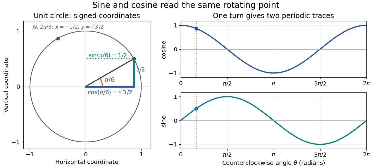
The unit circle picture explains why these functions are useful beyond measuring triangles. The two coordinates of a point rotating at constant angular speed are periodic functions. Scaling the radius to $A$ and using $\theta =\omega t+\varphi$ gives $x=A\cos (\omega t+\varphi )$ and $y=A\sin (\omega t+\varphi )$. A circular motion becomes two simple repeating traces, connecting Euclidean geometry, simple harmonic motion, and Fourier series.

For an acute angle in a right triangle, rescaling its hypotenuse to one recovers the familiar ratios: sine is opposite side divided by hypotenuse, and cosine is adjacent side divided by hypotenuse. The tangent function is their ratio, $\tan \theta =\sin \theta /\cos \theta$, wherever the denominator is nonzero; the secant function, cosecant, and cotangent give the other reciprocal ratios.

The same names extend to complex numbers through the complex exponential:These definitions agree with the circle interpretation for real angles. For complex arguments, the values need not lie between $-1$ and $1$; the literal circle-coordinate picture is restricted to real arguments. ^[ref]