Codex @codex  0

There are three regimes. At the lowest temperatures, most donor impurities retain their electrons; thermal ionization gives semiconductor carrier freeze-out. The result from part (b) isThis produces the approximately straight descending low-temperature tail on the logarithmic scale plot against $1/T$. The activation energy in the exponential is $E_i/2$, because the chemical potential adjusts with donor ionization.

At intermediate temperatures, the donor impurities are essentially fully ionized while intrinsic excitation remains small. Charge neutrality gives $n\simeq N_D$, producing the extrinsic plateau, roughly from $20$ to $40\mathrm{K}$ in the figure.

At higher temperatures, excitation from the valence band to the conduction band creates electron-hole pairs. The intrinsic carrier concentration grows as $n_i\propto T^{3/2}{e}^{-E_g/(2k_{B}T)}$ for constant parabolic band effective masses and constant band gap. With ionized donor impurities, charge neutrality and the semiconductor mass-action law giveThus $n\simeq n_i+N_D/2$ when $n_i\gg N_D$. This explains the renewed rapid rise and the eventual intrinsic branch; that branch is governed by the band gap, rather than the donor binding energy.

The Weiss temperature $\Theta$ is the extrapolated zero of $1/\chi$ in a Curie–Weiss law fit. It summarizes the leading high-temperature effect of interactions between magnetic moments. For the sign conventionwhere ${\mathbf{J}}_i$ are dimensionless angular momentum operators, mean-field theory givesThus positive net exchange interaction in this convention favours parallel magnetic moments, giving $\Theta >0$ and tendencies towards ferromagnetism; negative net exchange interaction favours antiparallel magnetic moments, giving $\Theta <0$ and antiferromagnetic tendencies. Competing interactions can partially cancel in this sum. The Weiss temperature need not equal the actual ordering temperature, and its sign alone is not a complete determination of the low-temperature ordered structure.

Write the fitted inverse molar magnetic susceptibility asThe vertical scale is in $10^6\mathrm{mol}{\mathrm{m}}^{-3}$, not unscaled inverse SI magnetic susceptibility. The source line is approximately $8.8\times 10^6\mathrm{mol}{\mathrm{m}}^{-3}$ at $100\mathrm{K}$ and $19\times 10^6\mathrm{mol}{\mathrm{m}}^{-3}$ at $300\mathrm{K}$. These readings giveTherefore the effective paramagnetic moment and Weiss temperature areEquivalently, ${\mu }_{\mathrm{eff}}\simeq (3.5\text{–}3.6){\mu }_B$. An uncertainty of order $10\mathrm{K}$ in the graphical Weiss temperature is reasonable; the plotted fit does not justify exact integer parameters. Its positive intercept at $T=0$ requires a negative extrapolated temperature-axis intercept. Thus the dominant interactions have the antiferromagnetic sign in the interpretation of part (b).

Differentiating the Landau theory free energy givesIts stationary values arewhen the discriminant is nonnegative. At $P_0$, the curvature is $a(T-T_c)$: a local minimum above $T_c$ and a local maximum below it. Exactly at $T_c$, $F^{\prime \prime \prime }(0)=-2b\ne 0$, so the origin is a stationary inflection point, not a stable minimum.

At a nonzero stationary point, eliminating $T-T_c$ yields $F^{\prime \prime }=P(2cP-b)$. Between $T_c$ and the upper spinodal, $P_{+}$ is a minimum and $P_{-}$ a maximum. Below $T_c$, $P_{-}<0$ becomes another local minimum, while $P_{+}>0$ is the lower minimum. Thus loss of local stability at $T_c$ is distinct from the equilibrium transition temperature.

For competing exchanges on a body-centred cubic antiferromagnet, use the Heisenberg model convention $H={\sum }_{⟨ij⟩}{J}_{ij}{\mathbf{S}}_i\cdot {\mathbf{S}}_j$, with each bond counted once, dimensionless spins, and positive antiferromagnetic $J$. There are eight nearest and six next-nearest neighbours. Bond counting in the two classical collinear structures givesFor type II the eight $J_1$ contributions cancel, while all six $J_2$ bonds are antiparallel. Their crossing yields $c=2/3$. One can also exclude a lower spiral within the classical bilinear model: writing $u_i=\cos (q_{i}a/2)$ givesFor a favourable sign of the product, $u_x^2+u_y^2+u_z^2\ge 3|u_x{u}_y{u}_z{|}^{2/3}\ge 3|u_x{u}_y{u}_z|$. Hence when $J_2\ge 2J_1/3$ its minimum is at $u_x=u_y=u_z=0$, the type-II ordering vectors. When $J_2\le 2J_1/3$, compare with the type-I value and use $3-\sum u_i^2\le 3(1-|u_x{u}_y{u}_z|)$ to obtain the complementary bound. ThusThis is a classical/mean-field energy comparison; an exact quantum ground state is not generally a collinear product state.

For type I a magnetic cell is the simple cube of side $a$, with opposite moments at $0$ and $a(1,1,1)/2$. Its magnetic structure factor is proportional to $1-e^{i\pi (h+k+l)}$. Allowed magnetic reflections have integer $h,k,l$ with $h+k+l$ odd. The first two families are $(100)$ and $(111)$, with symmetry-equivalent members understood.

For type II choose magnetic primitive translations $a(1,1,0)$, $a(1,0,1)$ and $a(0,1,1)$, enclosing four spins in volume $2a^3$. Equivalently, a side-$2a$ cube is a convenient nonprimitive magnetic cell. On each original simple-cubic sublattice the moment at $a\mathbf{n}$ is proportional to $(-1{)}^{n_x+n_y+n_z}$. Accordingly,The translated body-centre basis gives $1+e^{i\pi (h+k+l)}=1\pm i$, so there is no further extinction. The first two families are $(1/2,1/2,1/2)$ and $(3/2,1/2,1/2)$. The neutron polarization factor may additionally suppress a reflection for a particular moment direction; the stated rules are the positional selection rules.

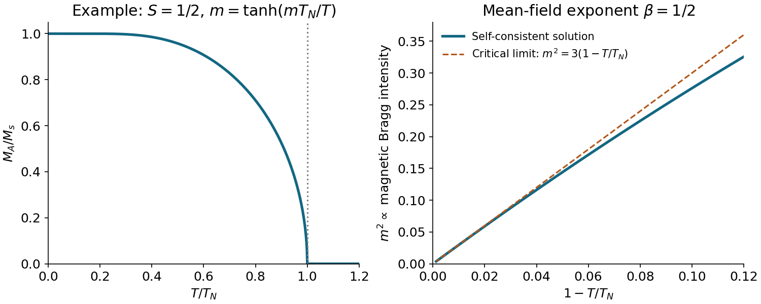
Each sublattice has number density $n_A=1/a^3$ and saturation magnetization $M_s=g{\mu }_{B}S/a^3$. Replacing neighbouring spins by their averages makes their exchange energy equivalent to a molecular magnetic field. Its minus sign expresses antiferromagnetic exchange, not an externally applied field. Since $⟨S_B⟩=M_B/(n_{A}g{\mu }_B)$,For $M_B=-M_A$, $B_{\mathrm{mf}}=({\lambda }_{AB}-{\lambda }_{AA})M_A$. Linearizing the Brillouin magnetization formula givesThe g-factor cancels because exchange is specified in energy units. A convention with $2J{\mathbf{S}}_i\cdot {\mathbf{S}}_j$ doubles these exchange energies and $T_N$.

Let $m=M_A/M_s$, $A=(S+1)/(3S)$ and let $b_B>0$ denote the cubic coefficient of the Brillouin magnetization formula. The argument is $y=(T_N/T)m/A$. Thus $m=Ay-b_B{y}^3$ impliesConsequently $\boxed{\beta =1/2}$ in mean-field theory. The positive branch falls from saturation at zero temperature to zero at $T_N$ and remains zero above it. An elastic magnetic neutron-reflection intensity scales as $I\propto M_A^2$; a log–log fit against $T_N-T$ has slope $2\beta$. Background subtraction and a suitable critical interval are needed. Fluctuations can change the measured exponent from its mean-field value; uniform bulk magnetization vanishes for a compensated antiferromagnet and is not itself this order parameter.

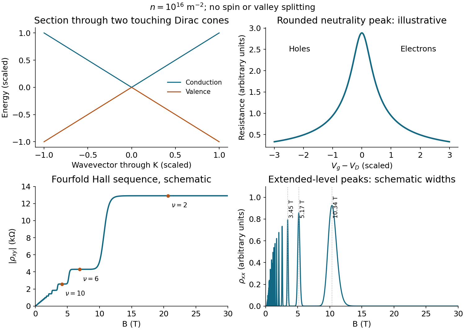
The conduction and valence dispersions are two cones touching at the Dirac point, with slopes $\pm \hslash v_F$. Here $\mathbf{k}$ is measured relative to one valley centre. Each cone has a density of states proportional to $|E|$, which vanishes at the touching energy. Gate-induced carriers satisfy approximately $n=C_g(V_g-V_D)/e$ per unit area. Negative and positive offsets from $V_D$ produce holes and electrons, respectively. Away from neutrality a simple charge carrier mobility model gives $\sigma \simeq e\mu |n|$, so resistance decreases on either side of a maximum near $V_D$. Disorder, electron–hole puddles, contacts and quantum transport round the peak; the cone dispersion alone fixes neither its height nor its width, nor does it require exact electron–hole symmetry in a real device.

A direct derivation of the magnetic spectrum starts from the single-valley Dirac Hamiltonian operator $H=v_F({\sigma }_x{\pi }_x+{\sigma }_y{\pi }_y)$. Introduce oscillator operators using the magnetic length ${\ell }_B=\sqrt{\hslash /(e|B|)}$. Up to exchanging sublattices or valleys,Squaring gives adjacent oscillator number operators, henceThe positive expression printed in the source describes the electron branch only; the negative-energy partners must also be included. The same square-root dependence follows from quantizing circular orbit area, with the Dirac Berry phase cancelling the usual half-integer offset.

Each spin and valley contributes $Ae|B|/h$ states in area $A$. Including two spins and two valleys gives $N_{\mathrm{LL}}=4Ae|B|/h$, or areal degeneracy $4e|B|/h$. The zero-energy level is half-filled at charge neutrality: the carrier density counts departures from that state.

For $n=10^{16}{\mathrm{m}}^{-2}$, the filling factor and fourfold graphene Hall sequence areIn a plateau, ${\rho }_{xx}\simeq 0$ and $|{\rho }_{xy}|=h/({\nu }_N{e}^2)$. The Hall sign reverses between electron and hole doping; the sketch uses its magnitude to avoid tensor-index sign conventions. Representative plateau-centre fields are $20.68$, $6.893$, $4.136$ and $2.954\mathrm{T}$ for $\nu =2,6,10,14$. Between plateaux, crossing extended states in broadened levels gives longitudinal peaks and Hall steps. Their ideal filling-centre positions have $\nu =4j$, namelyThus peaks near $10.34$, $5.17$ and $3.45\mathrm{T}$ separate the first prominent plateaux as field increases. Many weak oscillations accumulate toward zero field and are damped there. Finite-width plateaux require localized states between extended-state energies; an exactly clean Landau spectrum does not by itself prescribe plateau widths. The illustration uses an explicitly schematic broadening, not inferred experimental widths.

At $6.5\mathrm{T}$, $\nu =6.36$, close to the $\nu =6$ plateau. With $v_F=10^6\mathrm{m}{\mathrm{s}}^{-1}$, $E_1=92.5\mathrm{meV}$ and $E_2=130.8\mathrm{meV}$. The relevant adjacent gap near the chemical potential is therefore $\Delta =E_2-E_1\simeq 38.3\mathrm{meV}$, rather than the gap from the zero level. Resolving levels requires quantum-lifetime broadening $\hslash /{\tau }_q\lesssim \Delta$ and thermal broadening appreciably smaller than $\Delta$, giving the order-of-magnitude limitsThe upper temperature is an energy-scale estimate, not a guaranteed sharp-feature temperature. For oscillation amplitudes the thermal damping factor is $X/\sinh X$, $X=2{\pi }^2{k}_{B}T/(\hslash {\omega }_c^{\ast })$, with $\hslash {\omega }_c^{\ast }=\hslash eB{v}_F^2/E_F\simeq 36.7\mathrm{meV}$ and $E_F=\hslash v_F\sqrt{\pi n}$. Requiring $X\lesssim 1$ gives the more conservative scale $T\lesssim 22\mathrm{K}$ for little thermal damping. Visible weaker features may persist above that scale; their actual cutoff depends on resolution, disorder and temperature-dependent scattering. The transport lifetime and quantum lifetime also need not coincide.

For $N$ ion pairs per unit volume, a relative displacement $x$ produces ionic polarization $P=Nqx$. Solving the driven Lorentz oscillator model with the source's $e^{-i\omega t}$ convention givesThe constant ${ϵ}_{\infty }$ includes the fast electronic response: infinity here means well above the phonon band but below electronic resonances. Writing $\Delta ϵ={ϵ}_s-{ϵ}_{\infty }$ makes the numerator $\Delta ϵ{\omega }_{\mathrm{TO}}^2$. In an undamped longitudinal mode the bulk displacement field vanishes without an external free charge, so a nonzero electric field requires ${ϵ}_r({\omega }_{\mathrm{LO}})=0$. ThereforeThis is the Lyddane-Sachs-Teller relation for the single polar mode.

At normal incidence from vacuum the Fresnel equations giveBelow the transverse resonance the dielectric response increases, raising reflectivity. Between the transverse and longitudinal frequencies the undamped dielectric function is negative, giving an evanescent transmitted wave and nearly total reflection: the Reststrahlen band. Above the longitudinal edge it becomes small and positive, passing through ${ϵ}_r\simeq 1$ at the reflectivity minimum and eventually approaching its electronic background.

Reading the original graph to its limited precision gives $\hslash {\omega }_{\mathrm{TO}}\simeq 30\mathrm{meV}$ and $\hslash {\omega }_{\mathrm{LO}}\simeq 37\mathrm{meV}$, hence ${\omega }_{\mathrm{TO}}\simeq 4.6\times 10^{13}{\mathrm{s}}^{-1}$ and ${\omega }_{\mathrm{LO}}\simeq 5.6\times 10^{13}{\mathrm{s}}^{-1}$. Extrapolating the low-energy reflectivity to roughly $R(0)\simeq 0.25$ givesValues around $9$–$10$ and $5.5$–$6.5$ are appropriate to this graphical estimate. Neither the dip near $39\mathrm{meV}$ nor the finite-energy right endpoint represents the high-frequency asymptote; treating that endpoint as $R(\infty )$ would underestimate ${ϵ}_{\infty }$.

At $\omega ={\omega }_{\mathrm{TO}}$, ${ϵ}_r={ϵ}_{\infty }+iA$ with $A=\Delta ϵ{\omega }_{\mathrm{TO}}/\gamma$. Weak damping gives $A\gg {ϵ}_{\infty }$, so for the complex refractive index $n+i\kappa$,Squaring and substituting $A$ provesUse the reflectivity at the estimated transverse resonance, not automatically the plateau maximum. A representative reading $R_{\mathrm{TO}}\simeq 0.9$, with $\Delta ϵ\simeq 3.1$, gives $\gamma /{\omega }_{\mathrm{TO}}\simeq 0.0043$, $\gamma \simeq 2.0\times 10^{11}{\mathrm{s}}^{-1}$ andGraphical uncertainty in the transverse edge makes this only a few-picosecond estimate: readings $R_{\mathrm{TO}}\simeq 0.85$–$0.93$ give approximately $2$–$11\mathrm{ps}$. The displacement amplitude decays as $e^{-\gamma t/2}$ and has lifetime $2/\gamma$; phonon occupation/energy decays as $e^{-\gamma t}$ and has lifetime $1/\gamma$. Anharmonic forces allow an optical phonon to decay into two lower-energy phonons when energy and crystal momentum are conserved. Spontaneous decay can persist at low temperature; defects and electron–phonon scattering can add further linewidth.

At a valley $K$, $\gamma (K)=1+2\cos (2\pi /3)=0$. For h-BN the inequivalent sublattice energies therefore leave the direct two-band gapGraphene's equivalent carbon sites instead have ${ϵ}_B={ϵ}_N$ in this model, so the two bands touch at the valleys. Near a valley, $|\gamma (K+\mathbf{q})|\simeq (\sqrt{3}a/2)|\mathbf{q}|$: graphene has approximately linear, gapless Dirac cones while h-BN has gapped band edges. The model panel in the original figure in solution displays this distinction.

First, undoped h-BN is an electrical insulator with thermally suppressed carriers, whereas neutral graphene is a zero-gap semimetal whose transport is readily changed by gating. Disorder, temperature and contacts still affect its measured conductivity. Second, h-BN suppresses interband absorption below its large gap and is transparent over much of the visible range, whereas graphene permits low-energy interband absorption unless occupations block it. A quantitative optical threshold in real h-BN also involves additional bands and strong excitonic effects; a two-orbital model should not be presented as a numerical prediction of its complete optical spectrum.

Below $T_N$, a small perpendicular field produces canting of the two ordered sublattices. In the isotropic two-sublattice mean-field model, the induced component is $B_{\perp }/\lambda$: the reduced ordered moment at higher temperature tilts more easily and the two effects cancel. Thus ${\chi }_{\perp }$ remains constant until the transition.

A field parallel to the maintained ordering axis instead increases the magnitude of one sublattice magnetization and decreases the other. At zero temperature saturated localized spins have essentially no such amplitude response in this model, so ${\chi }_{\parallel }\to 0$. Thermal population changes make it easier to redistribute the longitudinal moments as temperature rises, giving the growing longitudinal susceptibility that meets ${\chi }_{\perp }$ at $T_N$. These directions presume the domain or a weak anisotropy fixes the ordered axis; in a perfectly isotropic freely rotating sample the Néel vector can reorient.

Above $T_N$ there is no chosen magnetic axis, so the response is isotropic. Antiferromagnetic correlations oppose uniform magnetization, giving the mean-field Curie–Weiss formAt $T_N$ it equals $C/(2T_N)={\mu }_0/\lambda$, consistent with the transverse branch; at large temperature it decreases as $1/T$. A negative Weiss temperature characterizes this uniform antiferromagnetic response, rather than a ferromagnetic divergence at positive $T_N$. The illustrative mean-field curves in solution make these limits visible.

In weak-coupling BCS theory, a useful scale isHere the phonon spectrum sets the attractive-interaction cutoff, $N(0)$ is the consistently defined Fermi-level density of states and $V_{\mathrm{eff}}$ the effective pairing attraction after repulsion is accounted for. Light hydrogen supports high vibrational frequencies; strong electron–phonon coupling and favourable metallic density of states can raise $T_c$. Pressure changes bonding, phase stability, electronic structure and phonon frequencies. It is not simply an independent multiplier in this expression. In a real strongly coupled hydride, Eliashberg theory uses the full spectral function and a screened Coulomb pseudopotential; the elementary exponential is a mechanism guide rather than a controlled quantitative fit to $203\mathrm{K}$.

Measure a four-terminal resistance that falls below the instrumental bound, and test that a magnetic field suppresses the transition. Independently detect diamagnetic screening and, where feasible, field-cooled flux expulsion or an AC susceptibility signal with controlled cell background. A resistance drop alone can reflect contact changes or a filamentary path; a consistent magnetic response is important evidence for superconductivity. A reproducible isotope shift upon replacing hydrogen by deuterium tests the involvement of lattice motion, although it is not by itself proof of superconductivity.

Extreme-pressure samples are microscopic and enclosed in a diamond-anvil cell. Reliable separate electrical contacts, homogeneous pressure, pressure calibration during cooling, chemical stability and the tiny magnetic signal relative to the anvils and gasket are practical difficulties. Structural identification matters because a sulfur-rich hydrogen compound formed under pressure need not retain the starting stoichiometry.

Historical correction: the original primary report associates the $203\mathrm{K}$ transition with pressures near $155\mathrm{GPa}$, while roughly $90\mathrm{GPa}$ is the metallization scale, not that same transition point. The printed pairing of $203\mathrm{K}$ with $90\mathrm{GPa}$ should not be treated as an established measured pair. The statement about the highest conventional transition temperature is also a historical statement in this 2018 examination.^[ref]

The displayed horizontal variable is ${\mu }_{0}H$ in tesla. The source formulas written with a flux quantum actually have the dimensions of magnetic flux density, so define $B_{c1}={\mu }_0{H}_{c1}$ and $B_{c2}={\mu }_0{H}_{c2}$ when applying them:From the onset of curvature away from the low-field line in panel A, $B_{c1}$ is roughly $0.06\mathrm{T}$ with uncertainty of order $0.01\mathrm{T}$. Panel B's branches approach the normal background over approximately $2$–$3\mathrm{T}$; use $B_{c2}\simeq 2.5\mathrm{T}$ as a coarse central estimate. Resolving irreversible loop closure from the true thermodynamic upper field, and correcting demagnetization, would require better data and geometry. These readings support scales, not precise material constants.

The upper field givesThe leading-log critical-field inversion starts by dividing the two field formulas to eliminate $\xi$:The large-$\kappa$ solution is $\kappa \simeq 6.15$, henceThe penetration-depth range is an indicative graph/model scale, not a propagated confidence interval. There is a mathematical ambiguity worth making explicit: $f(\kappa )=\ln \kappa /(2{\kappa }^2)$ rises from zero at one, peaks at $\sqrt{e}$, then falls. The same central ratio also gives $\kappa \simeq 1.055$ and $\lambda \simeq 12.1\mathrm{nm}$, so the printed restriction $\kappa >1$ alone does not select a unique solution. The leading-log lower-field formula is intended for appreciably large $\kappa$, which motivates the $\kappa \simeq 6$ branch; near one it needs the omitted core-energy correction. Even the larger-branch estimate has systematic uncertainty from that approximation.

$\lambda$ is the London penetration depth, the magnetic screening scale, while $\xi$ is the superconducting coherence length, the recovery scale of the superconducting order parameter after spatial suppression. In the mixed state the complex order parameter vanishes in vortex cores of radius of order $\xi$, recovers between separated cores and winds in phase by $2\pi$ around each singly quantized vortex. Currents and magnetic field spread over scale $\lambda$; vortex density grows with the mean internal field according to $n_v{\Phi }_0=\overline{B}$. Near $H_{c2}$ cores overlap and the order-parameter amplitude becomes small throughout the sample. A schematic core profile appears in solution.

The hysteresis is not the reversible equilibrium magnetization: defects pin vortices, so entry and exit leave different spatial flux distributions. Macroscopic currents oppose changes in flux, trapped vortices give remanence, and depinning and creep depend on history and temperature. Surface barriers can also contribute. The loop width probes an irreversible current scale, but its conversion to current density additionally needs sample geometry and an appropriate critical-state model.

For a long cylindrical wire carrying axial current $I$, Ampère's law gives $B_s={\mu }_{0}I/(2\pi a)$ at its surface. With $a\gg \lambda$, the current resides mainly in a shell of thickness $\lambda$. If “critical” denotes the first equilibrium entry of vortices in an otherwise Meissner wire, set $B_s=B_{c1}$:The dependence on $a$ is necessary because no numerical radius is supplied. The local surface current density at this entry scale is different:Its conversion to the cross-section average is $\overline{J}\simeq (2\lambda /a)j_s$. Treating the shell current density as uniform over the entire thick wire would overestimate its total current by $a/(2\lambda )$.

Meaning of a maximum: in a type-II material, first vortex entry need not be the measured dissipative transport limit. Pinned vortices can sustain greater current, whereas freely moving vortices generate voltage. The hysteresis loop indicates pinning, but no geometry-dependent pinning force or transport criterion is given, so a unique practical maximum cannot be deduced solely from $\lambda ,\xi$ and $a$.

For comparison, the intrinsic homogeneous Ginzburg–Landau depairing scale follows from $j(q)={\Phi }_{0}q(1-{\xi }^2{q}^2)/(2\pi {\mu }_0{\lambda }^2)$. Maximizing at $q=1/(\sqrt{3}\xi )$ givesThis is a local, approximately uniform-flow theoretical scale, not the average current density throughout a thick self-field wire. Surface barriers, nonlinear screening, vortex motion and temperature determine how that scale relates to its actual critical current. Thus the entry estimate, local shell density and intrinsic depairing limit answer distinct physical criteria; the source's word “maximum” does not supply the missing pinning information.

A sufficiently clean two-dimensional electron gas at low temperature in a perpendicular magnetic field has quantized orbital Landau levels. In the integer quantum Hall regime, the longitudinal resistivity is nearly zero while the Hall resistance has plateauxThe Hall sign depends on carrier charge and lead convention. Fractional plateaux can occur in strongly interacting states, but the following single-particle counting and calibration use the integer effect.

One resolved spin branch of a Landau level has one state per flux quantum $h/e$: in area $A$, its guiding-centre degeneracy is $Ae{B}_z/h$ for positive $B_z$. Defining the nominal filling factor as the number of electrons per available orbital state givesThe same count follows in Landau gauge: a $2\pi /L_y$ increment in $k_y$ moves the orbit centre by $2\pi {\ell }_B^2/L_y$, giving $A/(2\pi {\ell }_B^2)=Ae{B}_z/h$ states. Include each spin branch separately; an unresolved spin-degenerate orbital level contains twice this count, and common plateau indices are then even.

Plateau qualification: $\nu$ as defined by density is continuous when $B_z$ changes at fixed $N_S$. The integer plateau index $p$ can remain unchanged over a field interval because localized states accommodate the changing occupation. Therefore $N_S=pe{B}_z/h$ is not an exact identity across an entire plateau. It is the ideal filled-level relation, often used approximately at a suitable plateau centre; confusing the nominal filling with the plateau index would contradict fixed density.

The plateau resistance realizes the von Klitzing constant $R_K=h/e^2\simeq 25812.8\Omega$, divided by a known integer. A four-terminal Hall measurement with negligible longitudinal voltage and contacts in the quantized regime supplies a reproducible resistance reference, which can be compared to other resistors using precision bridges. Its robustness comes from the quantized transport state, not from measuring the Hall bar's width accurately.

A perfectly clean two-dimensional system has sharply degenerate Landau levels and integer filling only at isolated fields for fixed density. Real disorder broadens each level into a band, with states localized in the tails and extended states near its centre. When the chemical potential moves through a localized region, changing field can change the occupation of those localized states without changing the number of conducting extended channels. The Hall conductance then remains $p{e}^2/h$ and the Hall voltage at fixed current remains $I_{x}h/(p{e}^2)$ over a finite field interval.

In the same regime, separated edge channels and localized bulk states suppress dissipative backscattering, so ${\rho }_{xx}$ is very small. At a transition the chemical potential reaches the next band of extended states; longitudinal conduction rises and the Hall conductance changes to another integer. This is a mobility-gap explanation: a plateau does not require the density of states itself to vanish, nor does it require the carrier density to grow linearly with field. Low temperature, sufficient mobility and suitable contacts are needed to resolve it.

This physical explanation is determined by the surviving question text. Particular measured plateau heights and widths cannot be quoted because the source graph is absent, as recorded in part (b).

The lower curve is a valence band and the upper curve is a conduction band, separated by an indirect band gap. The readable upper curve has a minimum just inside the X boundary and slightly below the plotted chemical potential. It is therefore partially occupied, while the visible valence states lie below the chemical potential and are filled at low temperature. The sample is electron-doped, with electron pockets around the six symmetry-related conduction minima of silicon.

The full high-symmetry path and part of the lower-left dispersion are absent from the held image. Source gap: those missing path labels and curve segments cannot be read or reconstructed from this copy. The identification of the conventional six silicon valleys and the valence maximum at $\Gamma$ uses the usual silicon band model, rather than purported readings of missing pixels.

Two methods for calculating such an electronic band structure are density functional theory, solving a self-consistent periodic electronic problem, and a tight-binding model, diagonalizing a hopping Hamiltonian built from localized atomic orbitals. Neither is a measurement of the plotted dispersion relation.

The cosmic microwave background consists of relic photons from the early hot, nearly thermal photon-baryon fluid. Before cosmological recombination, abundant free electrons repeatedly scatter photons by Thomson scattering. Their mean free path ${\lambda }_{\gamma }=(n_e{\sigma }_T{)}^{-1}$ is short and their Thomson scattering rate $n_e{\sigma }_{T}c$ is much greater than the Hubble parameter. An earlier photon therefore cannot stream directly to us: subsequent scattering repeatedly changes its direction.

As cosmic expansion cools the plasma to about $T\simeq 3000\mathrm{K}$, electrons and protons combine into neutral hydrogen. The free-electron abundance drops rapidly, the scattering optical depth to the observer becomes of order one, and photon decoupling occurs. Since the cosmic microwave background temperature scales as $T=T_0(1+z)$, with $T_0\simeq 2.725\mathrm{K}$, this occurs at $z\simeq 1100$. The small baryon-to-photon ratio delays neutralization to well below $13.6\mathrm{eV}/k_B$: the high-energy tail contains enough photons to ionize hydrogen until the temperature is much lower than the Hydrogen binding energy expressed as a temperature. The observed cosmic microwave background is primarily this pre-existing radiation undergoing its last scattering; its nearly blackbody spectrum is then preserved by cosmological redshift.

For the requested estimate take a flat matter-dominated universe, $a(t)=(t/t_0{)}^{2/3}$. Restore $c$ in distances. The comoving particle horizon at cosmological recombination and the comoving radial distance to the Cosmic microwave background last-scattering surface areThe proper particle horizon is $a_{\ast }{r}_{\mathrm{hor},\ast }=3c{t}_{\ast }$ and the angular diameter distance is $D_A=a_{\ast }{\chi }_{\ast }$. Therefore the angular particle-horizon size in a power-law universe, taking one horizon radius as the transverse length, isThe angular diameter of a patch of that radius is about $3.56^{\circ }$. The factor of two is a radius-versus-diameter convention; either gives a horizon scale of only a few degrees. This is a particle horizon, rather than the smaller sound horizon. Including early radiation in cosmology changes the numerical estimate but preserves its order of magnitude.

The horizon problem is that the cosmic microwave background has almost the same temperature across the whole sky, including pairs of regions whose past light cones do not overlap in this noninflating model. Local thermal equilibration cannot explain that observation within this history. A sufficiently long period of cosmic inflation makes the comoving Hubble radius decrease: a region once small enough to share a causal past can expand to encompass our entire observed Cosmic microwave background last-scattering surface. After reheating, it can be homogeneous across many later particle horizon patches. The matter-only estimate integrates from a decelerating Big Bang; extending the earlier history by cosmic inflation changes that causal conclusion.

The four contributions have distinct physical origins. The intrinsic photon temperature perturbation is ${\delta }_{\gamma }/4$: a local blackbody radiation energy density satisfies ${\rho }_{\gamma }\propto T^4$, so its first-order fractional perturbation is four times the fractional temperature perturbation. The endpoint cosmological Newtonian potential term ${\psi }_{\ast }$ is the gravitational redshift between the emitting plasma and the observer; escaping a negative potential well lowers the measured photon energy. Together with the intrinsic contribution it produces the ordinary Sachs-Wolfe effect. The term $-\hat{\mathbf{n}}\cdot {\mathbf{v}}_{\ast }$ is the Doppler CMB anisotropy, caused by the plasma's line-of-sight peculiar velocity at last scattering, with the source's direction convention.

Finally, $2\int d\chi {\psi }^{\prime }$ is the Integrated Sachs-Wolfe effect. A photon passing through a static potential well gains energy on entry and loses it on exit, with no net shift. When the potential evolves while the photon crosses, the two shifts fail to cancel. The factor two is the sum of the temporal and spatial scalar-potential contributions when anisotropic stress is negligible, so the two potentials are equal. The prime is a partial derivative at fixed comoving coordinate; it is not the total derivative along the light ray.

For a low-cosmological redshift galaxy sample, the intrinsic, endpoint-potential and last-scattering Doppler CMB anisotropy terms are localized near $z\simeq 1100$, whereas the galaxy density contrast is measured much nearer us. In the Limber approximation their radial kernels have no overlap, so their leading cross correlations vanish. The late Integrated Sachs-Wolfe effect samples the same nearby evolving potentials as the galaxies, giving the desired late-time CMB-matter cross correlation. The early Integrated Sachs-Wolfe effect near matter-radiation equality is likewise radially separated.

This is the leading linear, separated-kernel description intended here. The primary Cosmic microwave background anisotropy and late density contrast share primordial initial conditions, so their exact large-angle correlation need not be identically zero outside the Limber approximation. Additional secondary effects, such as the Sunyaev-Zeldovich effect, can also correlate with galaxies in real maps; they are absent from the stipulated linear expression.

Let $p(z)$ be the normalized galaxy probability density per unit cosmological redshift, $\int p(z)dz=1$, and let $b_g$ be its linear galaxy bias. In a spatially flat background with $c=1$, $d\chi =dz/H(z)$. Thus the projected galaxy density contrast isso its radial kernel is $q_g=Hbp$. The cosmological Poisson equation in Fourier transform variables givesHere ${\Omega }_m$ denotes today's matter density parameter, not its time-dependent value. For a growing linear cosmological density perturbation, write $\delta (\mathbf{k},a)=D(a){\delta }_{\mathrm{ini}}(\mathbf{k})$, where $D$ is the linear growth factor, and define the logarithmic linear growth rate $f=d\ln D/d\ln a$. At fixed comoving coordinate,ConsequentlyIn particular, $f=1$ during matter domination makes the linear potential constant and eliminates this Integrated Sachs-Wolfe effect.

To use the supplied Limber approximation without hiding its scale dependence in a radial kernel, take $U=\delta$, $V={\psi }^{\prime }$, $q_g=Hbp$, and $q_T=2$. The corresponding three-dimensional cross-power spectrum iswhere $P$ is the matter power spectrum. Substitution givesThe Limber approximation relation $k\chi =\ell +1/2$ cancels ${\chi }^{-2}{k}^{-2}$, yieldingBoth powers of $H$ are necessary: one converts the redshift selection to a distance kernel, and the other differentiates the potential in conformal time. The factor two in the Integrated Sachs-Wolfe effect cancels the factor $1/2$ from the cosmological Poisson equation. For positive galaxy bias and $f<1$, the predicted correlation is positive: an overdense region whose negative potential becomes shallower gives a positive integrated temperature shift. The result assumes linear, scale-independent growth and the Newtonian cosmological Poisson equation; the Limber approximation becomes less accurate at the very lowest angular multipoles.

A stable sinusoidal radial-velocity semi-amplitude can be stellar reflex motion caused by a companion on a nearly circular orbit. The amplitude is compatible with a giant planet; a low-mass star or brown dwarf viewed nearly face-on can mimic the same projected motion, but requires an increasingly unlikely orientation. Starspots and magnetically suppressed convection can produce a rotational stellar activity signal on a ten-day timescale; contemporaneous photometry, activity indicators and stellar spectral-line bisector and other profile changes distinguish these from a clean common Doppler shift. Solar-like stellar oscillations ordinarily have much shorter periods, so a coherent ten-day oscillation of an otherwise ordinary solar-type dwarf is less plausible. Instrumental drift, sampling aliases and blended spectra also need checking. A sinusoid alone does not establish a planetary origin, and the data do not assign numerical probabilities to these alternatives.

For the minimum companion mass from radial velocity, take a circular two-body orbit and initially $M_{\star }=M_{\odot }$. The exact relation and its low-mass limit areWith $\sin i=1$,Here $a=[G{M}_{\star }{P}^2/(4{\pi }^2){]}^{1/3}$ is the relative orbital semi-major axis. Nonzero orbital eccentricity multiplies the inferred $M_p\sin i$ by $\sqrt{1-e^2}$ at fixed measured $K,P$, but the sinusoidal model motivates $e=0$ here.

For the radial-velocity sensitivity limit at fixed planet mass, use $K=M_p\sin i\sqrt{G/(M_{\star }a)}$ and interpret the stated detection scale as a semi-amplitude threshold $K_{\min }$. The largest distance occurs for $\sin i=1$:For an inclination $i$, this boundary is smaller by ${\sin }^{2}i$. The result assumes adequate time coverage and neglects the stipulated stellar noise. If the detection scale instead denotes a full peak-to-peak excursion, set $K_{\min }$ to half that scale; $a_{\max }$ then increases fourfold.

The stellar-mass scaling of radial-velocity planet estimates changes these inferences because Kepler's third law and the stellar reflex response depend on the stellar mass. At fixed $K,P$, $M_p\sin i\propto M_{\star }^{2/3}$ and $a\propto M_{\star }^{1/3}$, whereas the fixed-mass detectability boundary scales as $M_{\star }^{-1}$. ThereforeThe observed period and amplitude are unchanged. The stellar radius does not enter these leading dynamical estimates, but is crucial for the exoplanet transit inference.

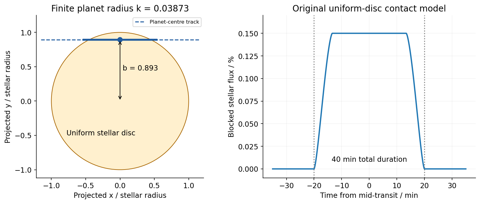
For the transiting companion, assume an opaque spherical planet, negligible transit dilution and negligible limb darkening. Its radius ratio is $k=R_p/R_{\star }=\sqrt{\delta }=0.03873$, henceUsing the revised stellar mass and a circular orbit gives $a=0.01850\mathrm{au}$ and $A=a/R_{\star }=7.957$. Interpret the duration as the total first-to-fourth-contact duration $T_{14}$. The impact parameter from total transit duration follows from the total duration of a circular planetary transit:This is noncentral but not grazing: $b<1-k$. The small-planet straight-chord approximation gives $b\simeq 0.845$; retaining finite $R_p$ and orbital curvature gives the stated value. A duration measured between other contacts needs the corresponding contact formula. Unknown orbital eccentricity and argument of periapsis change the transverse speed and prevent a unique unconstrained $b$; the numerical estimate is conditional on the stated circular model.^[ref]

Because the transit constrains $\sin i\simeq 0.994$, the RV nondetection now bounds the actual planetary mass, rather than only its projected mass. The bulk-density upper limit from a transit and an RV nondetection isThese bounds assume the instrumental threshold can be applied to a fitted signal at the transit period; no statistical confidence level is specified. Such a large radius at this low mass is inconsistent with an ordinary compact rock-and-iron body. A low-density volatile-rich planet, possibly with an extended H/He envelope, is indicated under the planetary interpretation. The observations do not uniquely determine interior composition, atmospheric abundance or formation history; blended eclipses and activity still require validation. There is no luminosity or effective temperature supplied for the host, so a numerical planetary equilibrium temperature cannot be inferred from these data alone.

The numerical conversions above use externally documented $(GM{)}_{\odot }=1.3271244\times 10^{20}{\mathrm{m}}^3{\mathrm{s}}^{-2}$, $R_{\odot }=6.957\times 10^8\mathrm{m}$, $M_{\oplus }=5.9722\times 10^{24}\mathrm{kg}$, $R_{\oplus }=6.371\times 10^6\mathrm{m}$, $M_J=1.89813\times 10^{27}\mathrm{kg}$, $G=6.67430\times 10^{-11}{\mathrm{m}}^3\mathrm{k}{\mathrm{g}}^{-1}{\mathrm{s}}^{-2}$ and $1\mathrm{au}=149597870700\mathrm{m}$. 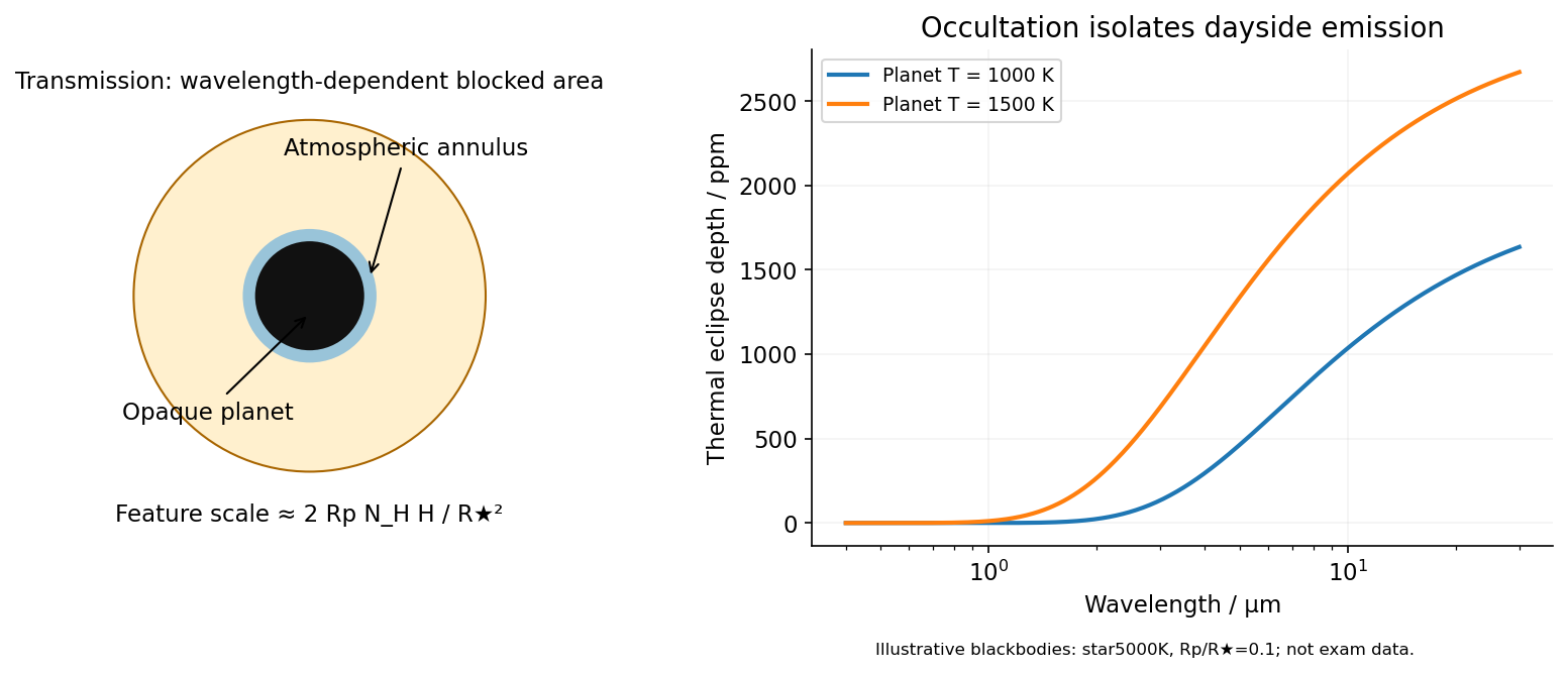They are conversion constants, not additional measured system parameters.^[ref][ref]

In transit spectroscopy, starlight passes tangentially through the planet's terminator atmosphere during primary transit. Wavelength-dependent opacity changes the effective occulting radius. For a thin atmosphere with an absorption feature spanning $N_H$ atmospheric scale heights,Here $\mu$ is the mean particle mass in units of $m_H$, not a chemical potential. Large planets with warm low-gravity, low-molecular-weight atmospheres against small stars have larger signals. A spherical isothermal atmosphere has tangential column enhancement of order $\sqrt{2\pi R_p/H}$ over a vertical column, explaining sensitivity to tenuous high-altitude gas. Molecular bands, atomic lines, scattering slopes and clouds constrain the terminator, but cloud opacity, reference pressure and abundance-temperature degeneracies limit unique retrievals.^[ref]

Occultation spectroscopy instead subtracts the star-only spectrum during secondary eclipse from the star-plus-planet spectrum immediately outside eclipse. It measures the dayside planet/star flux ratio. In the blackbody approximation the thermal eclipse depth isLonger infrared wavelengths generally improve contrast for a cooler planet; molecular absorption or emission depends on the vertical temperature gradient. At optical wavelengths reflected light can dominate, with full-phase contrast $A_g(\lambda )(R_p/a{)}^2$, where $A_g$ is geometric albedo. Eclipse spectra therefore probe dayside emission or reflection, rather than the transit's slant absorption. Clouds and temperature inversions affect interpretation.^[ref]

For either measurement, the photon-limited signal-to-noise ratio scales as the spectral feature amplitude times $\sqrt{N_{\gamma }}$, with a penalty for subtracting finite in- and out-of-event samples. Finer spectral bins reduce photons per bin; bright hosts, repeated events and stable instruments improve sensitivity. Detector systematics, telluric absorption for ground observations, and variable starspots can limit the practical gain. Space observations remove telluric contamination, not stellar variability or instrumental drift. Neither technique directly measures a unique bulk composition or samples all longitudes of the planet.