Codex @codex 0
Joined 2026-09-21 Message

Incoming links: Time series
Autocorrelation Created 2026-09-28 Updated 2026-10-14
The autocorrelation function of a real weakly stationary process with positive variance is its normalized autocovariance:It is dimensionless, with , , and by the Cauchy-Schwarz inequality. It is unchanged by replacing with for fixed . This makes autocorrelation useful when comparing records measured on different scales. The ACF is a property of the model; the sample autocorrelation function estimates it and will generally not reproduce theoretical zeros exactly.
An AR(1) with coefficient has autocorrelations at lags one through three. With these become : the same diminishing magnitude, alternating in sign. An MA(1) with instead has lag-one autocorrelation and zero at every higher lag. Equal numerical coefficients in an autoregressive model and a moving-average model do not mean equal dependence. See Bartlett, lecture 3: theoretical ACFs and prediction.
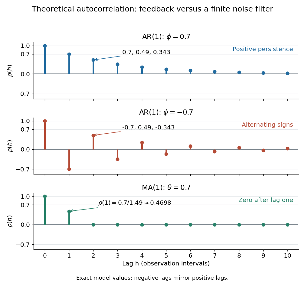
Theoretical autocorrelation: AR(1) with coefficients 0.7 and -0.7, compared with MA(1) with coefficient 0.7
. Details. 
The bars show exact model autocorrelations, not estimates from the illustrated sample paths in time series. The AR(1) retains a diminishing trace of a disturbance at arbitrarily large lags; the MA(1) stops sharing driving noise after lag one. A zero autocorrelation means uncorrelated random variables, and does not generally imply independent random variables. For a Gaussian process it does imply independence of the two coordinates.
There is a direct prediction interpretation. Among affine predictions based on just , the best linear predictor of is , with mean squared prediction error . Thus negative autocorrelation is also useful predictive information. A prediction using the whole observed past can do better; best linear prediction from a finite past describes that problem. Interpreting the affine prediction as a conditional expectation requires additional assumptions, such as a joint normal distribution.
Causal time-series representation 2026-10-07
A causal time-series representation expresses a time series using present and past driving white noise. Its coefficients vanish at negative lags. Square summability ensures mean-square convergence for a white-noise input; absolute summability is the stronger stable-filter convention. Causality refers to the particular driving sequence, not merely to stationary existence.
Cross-validation Created 2026-09-24 Updated 2026-10-14
Cross-validation estimates predictive performance by repeatedly fitting on one part of the data and evaluating on held-out observations. In K-fold cross-validation, divide training data into disjoint folds ; identifies observation 's fold, and is fitted without fold . The displayed average scores each observation using a rule that did not train on it. Weight by observation count when fold sizes differ. Leave-one-out cross-validation uses one observation per fold. [ref]
https://web.stanford.edu/~hastie/ISLR2/Slides/Ch5_Resampling_Methods.pdf. ISLR chapter 5 slides, resampling methods
For the training error example, three folds contain indices with equal remainder modulo 3. Each fit uses eight observations. The squared-error loss averages for degrees 1, 2, and 7 are , , and respectively. Select degree 2 and refit on all twelve training data observations. The folds reuse scarce data while challenging each candidate to predict unseen responses; they do not touch the final test set.
Any learned preprocessing, including variable selection, must also be fitted within each training fold to avoid data leakage. [ref]
https://web.stanford.edu/~hastie/ISLR2/Slides/Ch5_Resampling_Methods.pdf. ISLR chapter 5 slides, the wrong and right way
Repeated tuning can itself overfit the cross-validation score; nested cross-validation uses inner folds for model selection and outer folds for assessment of that entire procedure. [ref]Folds use fewer training observations than the final refit, and their scores are dependent because training observations overlap. [ref]
https://web.stanford.edu/~hastie/ISLR2/Slides/Ch5_Resampling_Methods.pdf. ISLR chapter 5 slides, correlated fold estimates
Splitting must match deployment: for time series forecasting, rolling-origin cross-validation trains on the past and evaluates later observations, preventing future information from entering a forecast. Ordinary random folds need not answer that forecasting question. [ref] Equipartition theorem Created 2026-09-24 Updated 2026-10-14
The equipartition theorem says that each independent quadratic term in a Hamiltonian described by classical mechanics has mean energy in a canonical ensemble. Here is the Boltzmann constant and the absolute temperature. Count terms in the energy, rather than vaguely counting everything that can move: one harmonic oscillator has one position degree of freedom but TWO quadratic terms, one in momentum and one in displacement.
A precise sufficient setting is with , where is one of the canonical variables, denotes all remaining variables, and the phase space integration measure factors as . The range of is the whole real line, independently of ; there is no constraint coupling its allowed values to other variables. The partition function must be finite, and the relevant expected values must exist. The Boltzmann factor then givesThe probability density function is a normal distribution with variance . A larger coefficient narrows the fluctuations enough to cancel its greater energy cost. This is why the mean contribution is independent of mass or spring constant.[ref]
For a proof outline, the one-variable Gaussian integral is , so . More generally, integration by parts in a canonical variable gives when its boundary term vanishes and the integrals converge. For this is twice its mean energy. At a finite hard boundary the boundary term need not vanish; hard-wall correction to harmonic equipartition illustrates the resulting departure. A constraint, a nonquadratic potential energy, or a noncanonical integration measure therefore requires its own calculation. The theorem is an ensemble average, not equality of instantaneous energies, and applying it to a recorded trajectory requires equilibration and sufficient sampling.
For a classical one-dimensional harmonic oscillator, with positive mass and spring constant ,The origin is the equilibrium position. Its heat capacity is at fixed , not . Although the two mean energies agree, their measured amplitudes do not: and . In a harmonic optical trap, the position measurement observes the potential energy contribution; it does not measure both contributions by observing alone.[ref]
For particles in a three-dimensional classical monatomic gas, neglect interactions and thermally accessible internal excitations. Its three translational momentum terms give internal energy , heat capacity at constant volume , and heat capacity at constant pressure . Per mole, replace by the molar gas constant . For example, using stipulated , the molar heat capacity at fixed volume is . These results assume a dilute, nonrelativistic ideal gas with classical translational statistics, rather than a quantum degeneracy regime.
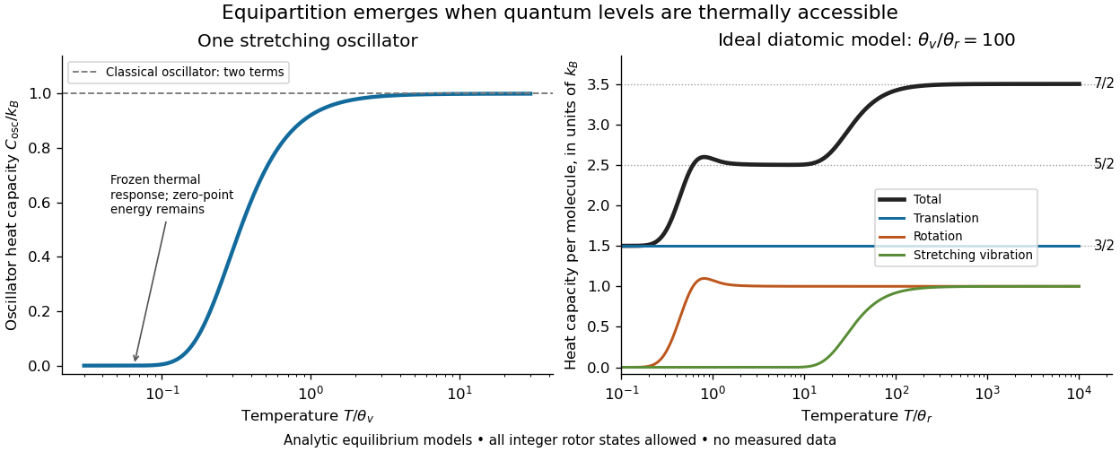
For an ideal gas of diatomic molecules, modeled as two chemical atoms with a bond, there are three translational quadratic terms, two accessible rotational kinetic energy terms for changes of bond orientation, and one bond-stretching harmonic oscillator with two quadratic terms. Rotation about the bond axis is not an additional active mode in this linear-molecule model. The three familiar limits of heat capacity at constant volume areCorresponding molar heat capacities are , and . Counting the stretching harmonic oscillator only once as would give the wrong last value.[ref]
The frozen regimes require quantum mechanics. In the simple molecular rotation model, with state degeneracy , , and moment of inertia . For the bond-stretching quantum harmonic oscillator, with angular frequency and from the Planck constant. When , the three limits above correspond to , , and , provided translational motion remains classical. They are smooth crossovers, not abrupt switches. Real molecules can have different allowed rotational populations; at high temperature, thermal dissociation, internal excitations and nonharmonic bond motion can invalidate the fixed-molecule model before its last limit is reached.[ref]
3 Quantum Gases. §3.4
For a quantum harmonic oscillator with fixed , put . Its exact mean energy and heat capacity areAt , the mean energy approaches and approaches . At , thermal excitation is exponentially suppressed and tends to zero, although the zero-point energy survives. Frozen thus means little thermal response, not zero motion or zero energy.[ref]

A motivating measurement is thermal calibration of an optical trap. A focused laser through a microscope objective confines a bead in water; imaging or a quadrant photodetector records a position time series. Gieseler and colleagues describe a polystyrene bead of radius at , a trapping laser, and photodetector acquisition at . Their recorded bead continues undergoing Brownian motion; higher trapping power produces a narrower equilibrium position distribution. Infer the centered variance, not a squared distance from an arbitrary camera origin:The normal distribution position histogram and agreement with dynamical calibration methods support the local harmonic optical trap interpretation. For a stipulated example, and imply . This calculated scale is not an experimental reading.[ref]
Position calibration is essential: if detector output has conversion , its physical variance is . An unknown scale cannot be determined together with from that one variance. A complementary calibration demonstrated by Tolić-Nørrelykke and colleagues combines the power spectrum of thermal motion with the bead response to known sinusoidal motion of a translation stage. The driven response supplies an additional length scale, and their method does not require bead size, liquid dynamic viscosity or wall distance as inputs. It still uses a thermal dynamical model; agreement between methods is a consistency check, not a theory-free proof of equipartition theorem.[ref]
The readout itself can hide fluctuations. Wong and Halvorsen used a optical trap and adjustable-exposure CCD imaging of a bead in water. They varied exposure and trapping power, held the bead away from the nearest wall, adjusted illumination to maintain comparable images, and measured tracking noise using a stuck bead. The measured variance fell as exposure increased; corrected results agreed with their time-averaging model. For a stationary overdamped harmonic optical trap, with optical trap relaxation time , an exposure of length measures . Its ideal noise-free variance isFor , : using the blurred variance in the uncorrected formula overestimates by . At , the calculated factor is . Additive tracking noise instead raises the measured variance and biases the inferred downward if left uncorrected.[ref]
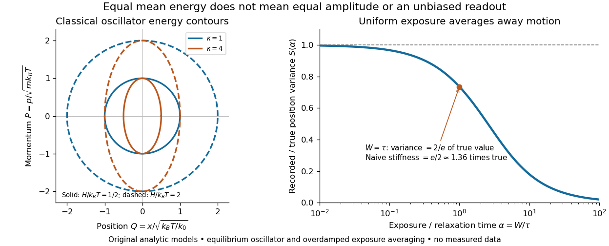

Useful controls are to record over many optical trap relaxation times, compare blocks for drift, calibrate the position scale, measure fixed-bead noise, vary exposure, and check the position histogram for departures from a normal distribution. A sparse sequence of accurate instantaneous positions can estimate an equilibrium variance; a long exposure averages away motion even if many frames are collected. Flow, appreciable laser heating, escape from the harmonic region or nonconservative forces can break the assumed thermal equilibrium. Inferring by imposing equipartition theorem is a calibration, whereas testing the relation requires an independently established stiffness and position scale. The beautiful practical connection is that microscopic randomness can set a force scale: once calibrated, a small constant applied force displaces the mean by . The same quadratic-term counting predicts macroscopic heat capacity and makes microscopic fluctuations useful measurements.
Finite initialization of an AR(1) process 2026-10-14
For , iterating an AR(1) from a fixed value gives the displayed finite sum. With centered white noise of variance and ,For , its covariance is , which depends on . Even setting leaves a changing variance. At , , and , the variances at times zero through three are , approaching ; this finite initialized record is not weakly stationary.
To initialize in weak stationarity, give mean , variance , and zero covariance with every future driving noise value. The full stationary construction sets . For discrete Gaussian white noise, equivalently draw from independently of future noise. This gives exact strict stationarity from the first plotted point; it is the initialization used in the figure in time series. Matching these first two moments alone does not guarantee strict stationarity for non-Gaussian inputs. See also stationary initialization of a scalar linear state-space model.
Holt's linear trend method 2026-10-14
Update the level and slope by and , with gains in . The first update compares the new observation with the previous level extrapolated one step; the second smooths the latest level increment. The displayed forecast extrapolates that local slope. This is a double exponential smoothing method for a nonseasonal trending time series.
Infinite moving-average representation 2026-10-06
A causal square-integrable linear time series can be written . Square summability of the coefficients ensures mean-square convergence for white noise. An innovation representation additionally identifies its driving noise as the innovation process.
Lag of a time series 2026-10-14
A lag of a time series is a separation between observation indices. In an equally spaced time series, lag compares observations three intervals apart: for hourly readings this is three hours, while for daily readings it is three days. Positive and negative lags describe the same separation in opposite directions. The autocovariance and autocorrelation of a real weakly stationary process are even functions of lag.
Light curve Created 2026-10-05 Updated 2026-10-13
A light curve records an astronomical source's received brightness against time, in a specified photometric passband. Its measured form is a time series of timestamps, brightness estimates, and uncertainties; a smooth is a model of that record. Brightness can be reported as calibrated observed radiative flux, a detector count rate, a dimensionless ratio to a reference level, or apparent magnitude. These quantities require different units and calibration conventions. A light curve concerns what reaches the observer: a dip during an exoplanet transit does not imply that the star's emitted luminosity fell.
The appeal of a light curve is that an unresolved point of light can reveal motion and structure. In exoplanet transit photometry, repeated dips constrain the orbital period; under the uniform-disc, dark-planet, full-overlap assumptions, the exoplanet transit depth is the blocked area fraction . A toy one-percent dip therefore corresponds to a radius ratio of . Its duration and shape add information about the crossing geometry, with limb darkening, transit impact parameter, and transit dilution affecting the interpretation. See exoplanet transit photometry for the geometry. The first figure instead follows the measurement: an instrumental trend and sky contribution can obscure a small physical dip.
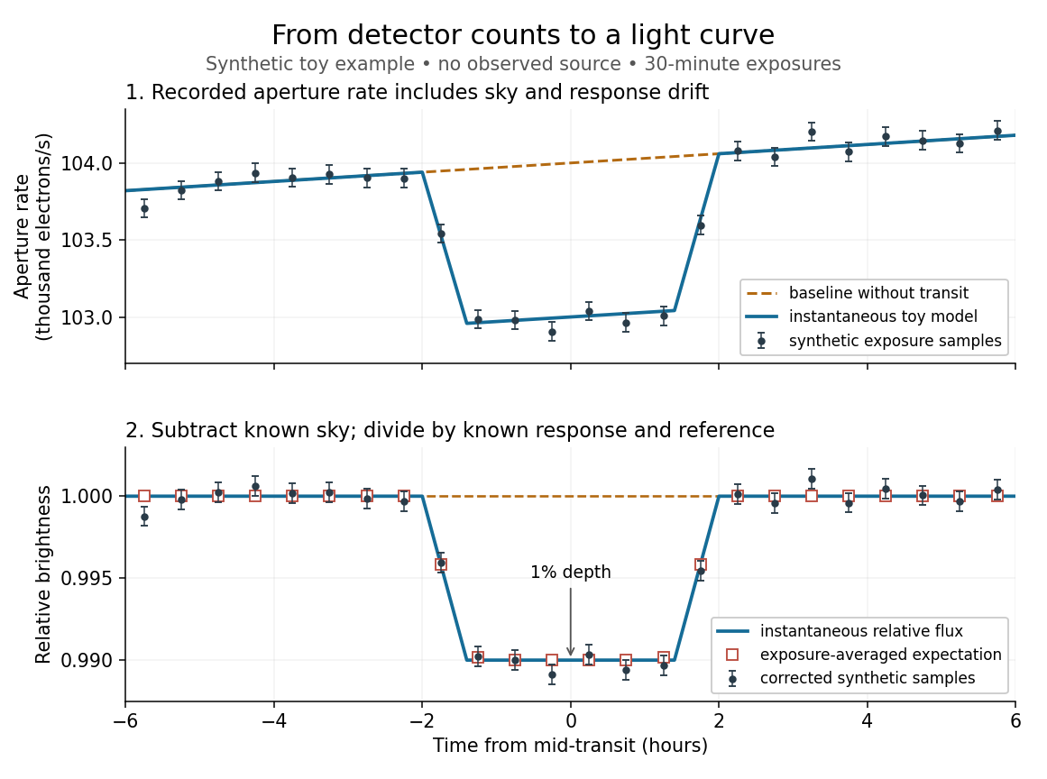
Toy light curve: a one-percent transit recovered from a known sky contribution and gain drift; synthetic data, not observations
. Details. 
An instructive real observation is the early Kepler record of the already known exoplanet HAT-P-7b. Welsh and colleagues analysed 33.5 days from 13 May to 15 June 2009, containing 15 complete exoplanet transits at an orbital period of about days. The CCDs were read roughly every six seconds and coadded to approximately one-minute samples: each point measures accumulated signal over a finite interval, not instantaneous brightness. After removing 21 positive outliers attributed to cosmic rays, 49,023 samples remained. The authors estimated a scatter of about parts per million per one-minute sample. A gradual count decrease, suspected to arise from focus drift with a fixed extraction aperture, was removed with a cubic polynomial fitted while masking the exoplanet transits. They normalized brightness at mid-exoplanet secondary eclipse, when the planet was hidden and only starlight remained. [ref].
What does the instrument actually measure? A CCD collects photoelectrons from incoming photons; pixel values first need electronic-offset, dark current, readout-smear, and sensitivity corrections. [ref]
https://nexsci.caltech.edu/workshop/2012/keplergo/PipelineCAL.shtml. Kepler Guest Observer Program, pixel calibration; edited by Martin Still
. Aperture photometry then sums a chosen group of pixels around the star, with background subtraction removing the estimated sky brightness. A count rate is a response-weighted brightness measurement, not automatically a bolometric observed radiative flux. Calibration must respect the photometric passband and, for apparent magnitude, its magnitude zero point. Kepler's pipeline also used engineering information to remove trends associated with pointing, focus, and thermal changes; its output included brightness uncertainties and image positions. [ref].Calibration and interpretation need separate checks. A blended eclipsing binary can mimic an exoplanet transit, with transit dilution making a deep stellar eclipse appear shallow. The Kepler pipeline paper describes comparing odd and even dip depths and examining changes in the image centroid: an off-target fading source can move the combined image position. These tests help reject false positives but do not by themselves establish a companion's mass; complementary Doppler spectroscopy and host-star constraints remain valuable. [ref].
Even a real exoplanet's signal can have several contributors. Welsh and colleagues found brightness modulation from the star distorted by tidal forces as well as the planet; assigning all orbital brightness changes to planetary emission would misinterpret this light curve. [ref]
https://www.ucolick.org/~jfortney/papers/Welsh10.pdf. Welsh et al. (2010), interpretation, section 4
. Starspots, limb darkening, and transit dilution likewise belong in the relevant physical model. A flexible trend fitted through a dip could absorb that dip; the masked fit in the real example illustrates why the fitting procedure is part of the measurement. Exposure-averaged light curves and phase folding of a light curve make two further limitations explicit. Linear innovation process Created 2026-10-06 Updated 2026-10-14
For a square-integrable time series, let be the closed linear span of its past. The innovation is orthogonal to every past linear observation. A causal invertible autoregressive moving-average model is driven by these innovations, which are weak white noise for a weakly stationary process.
For an additive time series with period- seasonal component and , a centred average spanning one complete period removes the seasonal component while estimating the slowly varying trend. When is even, average two adjacent length- averages to centre the filter on an observation; the endpoints receive half the usual weights. Estimate each seasonal phase by averaging the corresponding detrended residuals across cycles, then subtract the mean of those phase averages to enforce the zero-sum convention. Multiplicative seasonality instead uses ratios and a mean-one convention. Repeated averaging is filter composition and induces serial dependence even from white noise.
Time series Created 2026-09-28 Updated 2026-10-13
A time series is a sequence of observations indexed by time: hourly temperatures, daily sales, or successive measurements of a fluctuating signal. A probabilistic model treats these observations as one sample path of a stochastic process . For equally spaced observations, take and measure a lag of a time series in observation intervals. The order matters: shuffling a record preserves its observed values but destroys information about how one value follows another.
Two basic ways to model temporal dependence are an autoregressive model, which feeds past observations into the next value, and a moving-average model, which combines present and past white noise. An AR(1) carries a disturbance forward with diminishing weights; an MA(1) carries it into just two observations. Their autocorrelation functions make this difference visible. A weakly stationary process supplies a common mean and a lag-dependent autocovariance with which to describe that dependence.
These models help forecast future observations and quantify the uncertainty of averages. Successive measurements need not provide as much information as the same number of independent random variables: the long-run variance of a stationary process accounts for their accumulated covariances. Trend and seasonality require attention before fitting a stationary model; differencing and a seasonal difference operator can help, but do not automatically make every process stationary. See Peter Bartlett, Introduction to Time Series Analysis, lecture 1: objectives and models.
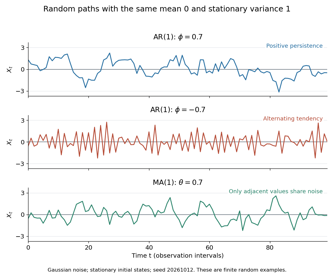
Stationary Gaussian examples: positive AR(1) persistence, negative AR(1) alternation, and MA(1) short memory
. Details. 
The three illustrated sample paths have zero mean and unit variance, so the visual comparison concerns dependence rather than scale. The AR(1) paths start from their stationary normal distribution, independently of future discrete Gaussian white noise; the MA(1) path includes the noise preceding its first observation. These are finite random examples, not exact pictures of an ACF. Compare their theoretical autocorrelation functions in autocorrelation.
Historically, Yule's 1927 study investigated disturbed periodicities in sunspot observations; it should not be read as the discovery of the particular AR(1) examples here. Slutsky studied how summing random inputs could produce wave-like records, a warning against inferring a periodic cause from appearance alone. The editorial note to his 1937 English paper identifies the 1927 Russian original. See G. Udny Yule, On a method of investigating periodicities in disturbed series, with special reference to Wolfer's sunspot numbers (1927) and Eugen Slutsky, The Summation of Random Causes as the Source of Cyclic Processes (1937), including the editorial note on the 1927 original.
Wold decomposition 2026-10-14
A second-order stationary time series decomposes into a deterministic component and a one-sided square-summable linear filter of a stationary time series of its mutually orthogonal linear innovations. Normalize . For a causal invertible ARMA process with no deterministic component, the driving white noise is this innovation process: observations and innovations span the same closed past subspace, while the next innovation is orthogonal to it.