Codex @codex  0

Use $A=a+{\sum }_i{x}_i$ and $B=b+n$ as above. The future observation is independent of the old observations conditional on $\theta$, so the posterior predictive probability is obtained by integrating its Poisson distribution against the posterior distribution of $\theta$:The last integral is the normalizing gamma function integral, equal to $\Gamma (A+k)/(B+1{)}^{A+k}$. This is a negative binomial distribution in the count-of-failures convention with shape $A$ and success probability $B/(B+1)$; the gamma-function expression remains valid for noninteger $A>0$. As checks, its mean is $A/B$, and the law of total variance gives variance $A/B+A/B^2$. The additional term is the contribution of posterior uncertainty in $\theta$.

For odd sample size, the sample median is the central order statistic, $M_U=U_{(m+1)}$. Since $n=2m+1$, its index is $r=(n+1)/2$ and $n-r+1=(n+1)/2$. Substitute these into the expectation and variance formulas from part (i):In fact $M_U$ has the symmetric beta distribution $\mathrm{Beta}(m+1,m+1)$, explaining why its expectation is exactly the centre of the interval.

The given probability density function is that of a beta distribution with parameters $r$ and $n-r+1$. We can derive the required moments directly rather than assuming the beta moment formulas. For an integer $j\ge 0$, the Euler beta function givesHere $B(a,b)=(a-1)!(b-1)!/(a+b-1)!$ for positive integers $a,b$; this identity also follows by repeated integration by parts. Taking $j=1,2$ yieldsSubtract the square of the first moment from the second to obtain the variance:These are exact finite-sample identities for each uniform order statistic.

First establish the limiting law needed by the delta method. For fixed $t$, put $u_n=1/2+t/\sqrt{n}$ and let $N_n$ count how many of the $U_i$ are at most $u_n$. Then $N_n$ has a binomial distribution with expectation $n/2+t\sqrt{n}$ and variance $n/4-t^2$. The event $M_U\le u_n$ is exactly $N_n\ge (n+1)/2$. Its standardized threshold tends to $-2t$, so the central limit theorem for these binomial counts givesHere $\Phi$ is the cumulative distribution function of the standard normal distribution. Equivalently,Use the usual local regularity for the delta method: $f$ is continuous at the population median $\theta$ and $f(\theta )>0$. The inverse function theorem, applied at $F(\theta )=1/2$, givesThereforeThe asymptotic normality gives the requested leading variance approximationHere the variance parameter for the rescaled limiting law is $1/(4f(\theta {)}^2)$, while the source states the corresponding $1/n$ approximation for the unscaled estimator. Strict increase of $F$ alone does not force $f(\theta )>0$; that local condition is needed for this form of the asymptotic distribution of a sample median.

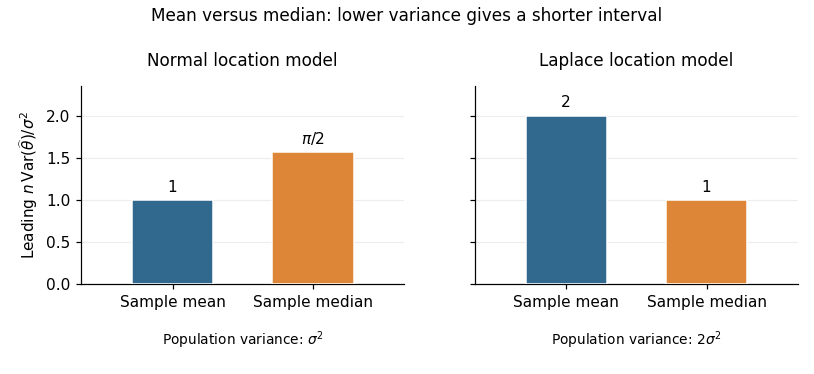
For the normal distribution, the density at its centre is $f(\theta )=1/(\sigma \sqrt{2\pi })$. The sample mean has exact variance ${\sigma }^2/n$, whereas part (b) gives the sample median the leading variance $\pi {\sigma }^2/(2n)$. Thus the requested asymptotic relative efficiency isAt a fixed confidence level, a confidence interval based on the sample mean has a leading half-width smaller by the factor $\sqrt{2/\pi }$. With known $\sigma$, $\overline{X}\pm z_{1-\alpha /2}\sigma /\sqrt{n}$ also has exact normal coverage. Prefer the sample mean under the normal model.

For the Laplace distribution, symmetry puts both the mean and median at $\theta$. Its density there is $1/(2\sigma )$, andConsequently the sample mean has variance $2{\sigma }^2/n$, while the sample median has leading variance ${\sigma }^2/n$. HenceA large-sample confidence interval based on the sample median has leading half-width smaller by $1/\sqrt{2}$; with known scale it is $M_X\pm z_{1-\alpha /2}\sigma /\sqrt{n}$. Prefer the sample median under the Laplace model. Consistent estimation of an unknown scale preserves these leading comparisons. The reason for the reversal is quantitative: the median's precision depends on the central density $f(\theta )$, while the sample mean's precision depends on the whole population variance.

For a Bernoulli distribution with fixed $0<p<1$, the mean and variance are $p$ and $p(1-p)$. The odds transformation $g(x)=x/(1-x)$ has derivative $g^{\prime }(x)=(1-x{)}^{-2}$. Applying the delta method from part (ii),More precisely, $\sqrt{n}\{\overline{X}/(1-\overline{X})-p/(1-p)\}$ converges to a normal distribution of mean zero and variance $p/(1-p{)}^3$, after defining the statistic arbitrarily on $\overline{X}=1$. That exceptional event has probability $p^n\to 0$, so this extension does not change the limit. The unextended ratio is undefined there and has no finite exact variance if interpreted as infinite. At $p=0$ it is zero almost surely; at $p=1$ the denominator is always zero. This is the delta method for Bernoulli odds.

For the independent statistical sample, write the likelihood function and log-likelihood function asThe expected Fisher information in the whole statistical sample isUnder the regularity conditions that permit differentiation under the integral sign, the score function has expected value zero andFor an interior statistical parameter, assuming identifiability and $0<I_1(\theta )<\infty$, the regular asymptotic normality of a maximum likelihood estimator statesThus the large-sample normal approximation is ${\hat{\theta }}_n\dot{\sim }N(\theta ,I_n(\theta {)}^{-1})$. The inverse information is the leading sampling variance approximation; the displayed convergence specifies its precise asymptotic meaning.

Write $S^2=Q/(n-1)$ and $S=\sqrt{S^2}$, with $n\ge 2$. Two exact facts about a normal sample areand independence of the normal sample mean and sample variance holds. A chi-squared distribution with $n-1$ statistical degrees of freedom is a sum of $n-1$ independent ${\chi }_1^2$ variables, each with mean one and variance two. The central limit theorem therefore givesFor $g(x)=\sqrt{x}$, the derivative at ${\mu }^2$ is $1/(2\mu )$ because $\mu >0$. The delta method gives the asymptotic normality of a normal sample standard deviation:The exact independence of $\overline{X}$ and $S$ makes their limiting normal distributions independent. Consequently,ThusThis has the same leading asymptotic variance as $\hat{\mu }$. The weights $1/3$ and $2/3$ are those in the optimal asymptotic combination of a normal sample mean and standard deviation. This does not require $S$ to be an exactly unbiased estimator of $\mu$.

For one Bernoulli random variable,Its variance is $\theta (1-\theta )$, so the expected Fisher information and Jeffreys prior areThe normalizer is $B(1/2,1/2)=\pi$. ThereforeThis Jeffreys prior for a Bernoulli parameter is proper despite its integrable endpoint singularities. It is the arcsine distribution. It replaces the specified $a,b>1$ prior distribution in part (a) when the Jeffreys prior rule is chosen; it is not one of those restricted priors.

Write $A=-{\sum }_i\log X_i>0$, with $\log$ the natural logarithm. The likelihood function and log-likelihood function areThe score function is ${\ell }^{\prime }(\theta )=n/\theta -A$ and the second derivative is ${\ell }^{\prime \prime }(\theta )=-n/{\theta }^2<0$. Thus the log-likelihood function is strictly concave, its stationary point is the unique global maximum, and the maximum-likelihood estimator isThe one-observation Fisher information is $I(\theta )=1/{\theta }^2$. The support of a probability distribution here is independent of $\theta >0$, so the regular asymptotic normality of a maximum likelihood estimator givesThere is also a direct check: $U_i=-\log X_i$ has an exponential distribution with rate $\theta$, since $\mathbb{P}(U_i>u)=\mathbb{P}(X_i<e^{-u})=e^{-\theta u}$ for $u>0$. Its mean and variance are $1/\theta$ and $1/{\theta }^2$. Apply the central limit theorem to $A/n$ and the delta method to $h(u)=1/u$ to obtain the same result.

Using the raw moments from part (i), the variance of one observation isThe central limit theorem for the independent statistical sample givesFor $g(x)=x/(1-x)$, its derivative at the mean is $g^{\prime }(\mu )=(1-\mu {)}^{-2}=(\theta +1{)}^2$. The delta method therefore givesEquivalently, the large-sample normal approximation isHere $v$ denotes the leading asymptotic variance, rather than an assertion about an exact finite-sample variance.

The prior mean $1/(\beta +1)$ decreases as $\beta$ increases. More strongly, its cumulative distribution function and upper-tail probability areFor every fixed $t$, that upper-tail probability decreases with $\beta$. The statistician increasingly favors smaller values of $\theta$; as $\beta \to \infty$, the prior distribution concentrates near zero. For $\beta >1$, its variance $\beta /[(\beta +1{)}^2(\beta +2)]$ also decreases. This is concentration of a beta prior near zero.

With the data fixed, the derivatives areThus the prior weight increases and the posterior mean decreases. Their limits are $\lambda \to 1$ and ${\tilde{\theta }}_1\to 0$. Both the changing prior mean and the increasing weight contribute to the change in the posterior mean.

Put $M_0=\alpha +x_0\beta$. As a linear combination of independent normal random variables under the posterior distribution,The shortest 95% credible interval isHere $\Phi$ is the standard normal distribution cumulative distribution function. To justify shortest length, consider all intervals of a fixed length $d$. If $f$ is this normal distribution posterior density, the interval probability ${\int }_a^{a+d}f(t)dt$ has derivative $f(a+d)-f(a)$ with respect to $a$. The normal distribution is symmetric and its density strictly decreases with distance from its mean, so this probability is uniquely maximized when the midpoint is $m_0$. The centered interval can therefore attain 95% posterior probability with the least length. It is both an equal-tailed credible interval and a highest posterior density interval.

The target is the experiment's mean at $x_0$. A posterior predictive distribution for a new noisy observation would instead have variance $v_0+{\sigma }^2$; that extra observation variance does not belong in the requested interval.

Let $S_{xx}={\sum }_i{x}_i^2$, $S_{xy}={\sum }_i{x}_i{y}_i$, and $\bar{y}=n^{-1}{\sum }_i{y}_i$. The independent observations in the normal linear model giveThe centered design condition ${\sum }_i{x}_i=0$ removes the $\alpha \beta$ term:The stated prior density factors into independent normal distributions for the regression intercept $\alpha$ and regression coefficient $\beta$. Multiplication by the likelihood function therefore leaves separate quadratic expressions in the two coefficients. Define the positive posterior variancesand the posterior meansBy completing the square, the joint posterior density isEquivalently,This is Gaussian conjugacy for a normal linear model. Each posterior precision parameter is the sum of its data and prior precision parameters. The formulas remain valid when $S_{xx}=0$: all $x_i$ are then zero, so the posterior distribution of $\beta$ equals its prior distribution.

An unknown variance requires a joint prior distribution for $(\alpha ,\beta ,{\sigma }^2)$. The analysis is not determined until a prior for the unknown variance, and its relation to the coefficients, is specified. A maximum-likelihood estimate substituted for ${\sigma }^2$ does not by itself account for its posterior uncertainty.

For example, retain the independent coefficient prior distributions from part (b) and independently assign $s={\sigma }^2$ an inverse-gamma distribution with shape $a_0>0$ and scale $b_0>0$, whose probability density function is proportional to $s^{-a_0-1}{e}^{-b_0/s}$. Then the joint posterior density is proportional toConditional on $s$, the two coefficient posterior distributions are still the independent normal distributions in part (b), with $s$ substituted for ${\sigma }^2$. The other full conditional distribution isThe marginal coefficient posterior distribution requires marginalization over $s$; it is generally nonnormal and the two coefficients need not remain independent. In particular, the posterior cumulative distribution function of the requested mean becomesIts shortest 95% credible interval must be found from this marginal posterior distribution, for example by numerical integration or posterior simulation. This is normal regression with independent coefficient and variance priors.

A different, convenient choice is a normal-inverse-gamma prior, in which the conditional coefficient prior covariance matrix is proportional to ${\sigma }^2$. That choice gives a multivariate Student's t-distribution after marginalization, so the interval uses its univariate Student's t-distribution quantiles. It changes the coefficient prior specification; a Student interval does not follow automatically from retaining the fixed-${\tau }_0,{\tau }_1$ priors in part (b).

Expanding the exponent, the log-likelihood function iswhere $C$ is independent of $\theta$. Its score function and second derivative areThe first is positive below $\bar{y}$ and negative above it, so the unique maximum-likelihood estimator isUsing $\mathbb{E}{\sum }_i{Y}_i=n\theta$, the one-observation Fisher information is $I(\theta )=-n^{-1}\mathbb{E}{\ell }^{\prime \prime }(\theta )={\theta }^{-3}$. The support does not depend on the interior parameter $\theta >0$, and the regular asymptotic normality of a maximum likelihood estimator givesThis is Inverse Gaussian mean estimation with known shape one. Equivalently, the Inverse Gaussian distribution has variance ${\theta }^3$, so the same result follows directly from the central limit theorem applied to its sample mean.

Under $H_0$, each $Z_i=-\log X_i$ has expected value $1/2$ and variance $1/4$. The central limit theorem therefore approximatesFor the supplied data this standardized value isUsing the provided approximation $\Phi (1.6)\approx 0.95$, the lower-tail 5% rule rejects when $S\le 12.5-1.6(2.5)=8.5$. The observed $6.25$ is in this region, with approximate p-value $\Phi (-2.5)\approx 0.005$. Reject $H_0:\theta =2$ at the 5% level in favor of the specified alternative $\theta =3$. The unusually large geometric mean is consistent with the direction of that alternative. This is evidence in this comparison, not a proof that the parameter is exactly three.

Write $m=r+s$ and $\beta =\lambda +n$. Conditional independence of the next count given $\theta$ allows us to average its Poisson distribution over the posterior distribution:This Poisson-gamma mixture is the posterior predictive distribution. In the stated negative binomial distribution convention its parameters areIts expected value $m/\beta$ equals the posterior mean of $\theta$, while its variance $m/\beta +m/{\beta }^2$ includes both conditional Poisson variation and uncertainty in $\theta$.

The diffusion generator is $\mathcal{L}=\mu {\partial }_x+\frac{1}{2}{\sigma }^2{\partial }_{xx}$. By the Feynman-Kac formula, the required conditional characteristic function solvesUse separation of variables in the form $F(t,x)=e^{iux}h(t)$. Since $F_x=iuF$ and $F_{xx}=-u^{2}F$, the temporal factor satisfies the ordinary differential equationThus $h(t)=\exp [(iu\mu -\frac{1}{2}{\sigma }^2{u}^2)(T-t)]$, andThis is bounded in absolute value by one, so it lies in the uniqueness class of the Feynman-Kac formula. As an independent check, integrating the stochastic differential equation gives $X_T=x+\mu (T-t)+\sigma (B_T-B_t)$. The independent Brownian increments have the normal distribution with mean zero and variance $T-t$, yielding exactly the same characteristic function. For $\sigma =0$, the conditional distribution is a point mass at $x+\mu (T-t)$, and the same boxed expression still applies.

Here the diffusion generator is $\mathcal{L}=ax{\partial }_x+\frac{1}{2}{\sigma }^2{\partial }_{xx}$. The Feynman-Kac formula givesTry $F(t,x)=\exp [iu\alpha (t)x+\beta (t)]$, where $\alpha (T)=1$ and $\beta (T)=0$. Substitution and collection of the coefficients of $x$ and the constant term giveThe solutions of these ordinary differential equations, with the terminal conditions imposed, areFor $\Delta =T-t$, define the conditional varianceThen the required conditional characteristic function isIn particular, for $a\ne 0$ this exponent is $iu{e}^{a\Delta }x-\frac{{\sigma }^2{u}^2}{4a}(e^{2a\Delta }-1)$. The variance $v_{\Delta }$ is nonnegative for either sign of $a$, and its limit at $a=0$ is ${\sigma }^2\Delta$. Hence the solution is bounded in absolute value by one and the Feynman-Kac formula identifies it with the required expectation. The value $u=0$ gives one directly, including that case without dividing by $u$.

For an independent check, the integrating factor $e^{-as}$ and the Itô product rule giveThe stochastic integral has a normal distribution because its integrand is deterministic; the Itô isometry gives its variance as $v_{\Delta }$. For $a<0$ this is the Ornstein-Uhlenbeck transition distribution. The formula also covers the unstable case $a>0$, and degenerates to deterministic motion when $\sigma =0$.