Codex @codex  0

The variance of a predictive distribution quantifies spread of a future quantity conditional on the observed data and model assumptions. For a noisy future observation $Y_{\ast }=f_{\ast }+{ϵ}_{\ast }$ with fresh independent noise of variance ${\sigma }^2$, it is $\mathrm{Var}(f_{\ast }\mid \mathcal{D})+{\sigma }^2$. It should therefore be distinguished from the latent-function posterior variance.

Preparation uncertainty describes the outcome spread intrinsic to a specified quantum state preparation. Operationally, prepare many copies of the same quantum state, measure position on one group and momentum on another, and estimate the two variances. Ideal measurements still have the spreads predicted by the Born rule. No earlier position measurement need occur in the momentum group. The Heisenberg uncertainty relation constrains these two distributions belonging to the same preparation.

Measurement backaction concerns how a particular measurement in quantum mechanics changes a quantum state. Instrument resolution concerns how its reported outcomes relate to the intended observable. Those questions require a model of the instrument and its interaction with the system. Substituting an instrument error and an induced change for $\Delta x$ and $\Delta p$ in the Heisenberg uncertainty relation does not follow from its proof. The practical value of preparation uncertainty is that it bounds achievable input spreads before any such instrument model is chosen.

For positive marginal variances, standardizing each variable to variance one converts covariance-based PCA on $Z$ into correlation-based PCA on $X$. This makes the analysis insensitive to the original measurement units but changes the optimization criterion. Standardization gives small-variance variables the same marginal weight as large-variance variables; it is a modelling choice, not an automatic improvement.

A score is an observation's coordinate along a principal component direction. Center an observation by the fitted sample mean, apply the fitted variable scaling when using principal component analysis on a correlation matrix, then take its inner product with the unit principal component loading vector. New observations must use the training center and scaling. The score variance equals the corresponding eigenvalue when the covariance normalization is consistent.

Prior probability describes uncertainty before the current observations are incorporated. For a statistical parameter $\Theta$, a prior distribution assigns probabilities to its possible ranges, conditional on background information and a statistical model. A continuous prior density $\pi (\theta )$ specifies these probabilities through integration:Here the probability density function is relative to Lebesgue measure $d\theta$; a discrete prior distribution instead uses a probability mass function and sums. Density at one point is not the probability of that point. A nonnegative kernel with infinite total mass is an improper prior, whose use requires a separate check of posterior propriety.

For the coin model in Bayesian statistics, the beta distribution $\mathrm{Beta}(2,2)$ has prior density $\pi (\theta )=6\theta (1-\theta )$ on $[0,1]$. Its mean is $1/2$ and its variance is $1/20$. It favors moderate heads probabilities without ruling out values near zero or one. For example,The prior curve in Bayesian posterior makes this preference visible; moment matching for a beta prior explains how to choose a beta distribution from a desired mean and variance.

A prior distribution lets earlier evidence or elicited knowledge contribute to statistical inference when the current sample size is limited. It also exposes assumptions that can be checked by prior elicitation and a prior predictive check. Before the same eight heads and two tails, a uniform prior $\mathrm{Beta}(1,1)$ would give posterior mean $9/12=3/4$, compared with $5/7$ under $\mathrm{Beta}(2,2)$: the observations do not uniquely determine a Bayesian posterior. Even a uniform prior makes a choice of parameter coordinates; its child article explains why changing coordinates can destroy uniformity.

Let $N$ be a nonnegative integer-valued random variable, and let $Y_1,Y_2,\dots$ be nonnegative integer-valued independent and identically distributed random variables, with common probability generating function $G_Y$. Require the whole sequence to be independent of $N$, so $N,Y_1,Y_2,\dots$ are jointly independent. Set the random sumwith the empty sum equal to zero. Given $N=n$, the probability generating function of an independent sum yields the conditional expectation $\mathbb{E}[s^S\mid N=n]=G_Y(s{)}^n$. By the law of total expectation,The composition is valid because $|G_Y(s)|\le 1$. Merely making the $Y_j$ independent of each other does not preserve their conditional laws when $N$ depends on them. This is the probability generating function version of transform composition for an independent random sum.

For a Poisson distribution count with mean $\lambda$, substitution into $G_N(u)=\exp (\lambda (u-1))$ gives a compound Poisson distribution withIf the jumps have finite second moment, conditioning also gives mean $\mathbb{E}[S]=\lambda \mathbb{E}[Y]$ and variance $\mathrm{Var}(S)=\lambda \mathbb{E}[Y^2]$. The extra spread comes from randomness in the count as well as randomness in the jumps.^[ref]

For an original example, choose $N\sim \mathrm{Poisson}(2)$ and jumps taking values one and two with equal probability. Keep the independence assumptions above. ThenHere $\mathbb{E}[Y]=3/2$, $\mathrm{Var}(Y)=1/4$, and $\mathbb{E}[Y^2]=5/2$. The law of total expectation and law of total variance giveThus the aggregate is not itself a Poisson distribution, whose mean and variance would coincide.

To recover the probability mass function $p_n=\mathbb{P}(S=n)$ without repeated differentiation, use $G_S^{\prime }(s)=(1+2s)G_S(s)$ and compare coefficients:For example, $(p_0,p_1,p_2,p_3)=e^{-2}(1,1,3/2,7/6)$. As an independent check, expanding $e^{s+s^2-2}=e^{-2}{e}^s{e}^{s^2}$ gives

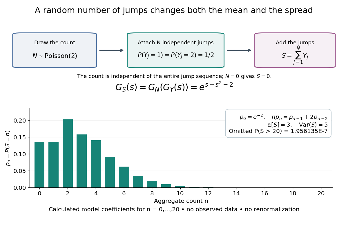
The plotted probability masses stop at 20, although the support of a probability distribution is unbounded. The omitted tail probability isThis model has bounded jumps and an unbounded count. Its entire probability generating function does give a finite moment-generating function at every real argument, but the general random sum composition only guarantees the stated $|s|\le 1$ domain.

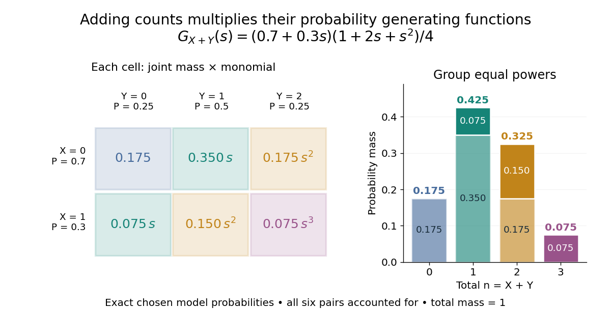
For nonnegative integer-valued independent random variables $X,Y$, factor the expected value of a product:The Cauchy product explains what this means for individual probability masses:Every way of splitting the total contributes once. This is convolution of independent random variables; multiplying probability generating functions performs the bookkeeping automatically.

For an original example, take independent $X\sim \mathrm{Bernoulli}(0.3)$ and $Y\sim \mathrm{Binomial}(2,0.5)$, using the Bernoulli distribution and binomial distribution. ThensoDirect enumeration of the six pairs $(x,y)$ gives the same probability masses. For example, total one collects $(0,1)$ and $(1,0)$, with contributions $0.7\cdot 0.5+0.3\cdot 0.25=0.425$. The coefficients sum to one. The expected value is $G_{X+Y}^{\prime }(1)=1.3$; since $G_{X+Y}^{\prime \prime }(1)=1.1$, the variance is $1.1+1.3-1.3^2=0.71$, agreeing with $0.3\cdot 0.7+2\cdot 0.5\cdot 0.5$.

Uncorrelated random variables are insufficient for the product identity. For a concrete counterexample, let $U$ be uniform on $\{-1,0,1\}$ and set $A=U+1$, $B=U^2$. Then $\mathrm{Cov}(A,B)=\mathbb{E}[U^3]=0$, but $\mathbb{P}(A+B=0)=0$, whereas $G_A(0)G_B(0)=1/9$. Zero covariance controls one mixed moment, not the full joint probability mass function.

Probability inequalities bound event probabilities from limited information, such as moments, without requiring a complete probability distribution. Markov's inequality uses a nonnegative random variable's expected value; Chebyshev's inequality uses a variance to bound deviations from a mean. The attraction is a guarantee that applies to many possible probability distributions. Their bounds can be conservative for a particular model, and distributions attaining equality show when the available information really cannot give more.

Probability theory describes uncertainty through a probability space: possible outcomes form a sample space, observable questions are events, and a probability measure assigns them numbers between zero and one. The Kolmogorov axioms make those assignments consistent. They let us combine information about several events, update it through conditional probability, and study random variables without listing every possible outcome separately.

For example, roll two dice whose results are independent random variables, each with a discrete uniform distribution on $\{1,\dots ,6\}$. There are 36 equally likely ordered outcomes. Only $(1,6),(2,5),\dots ,(6,1)$ have sum seven, so that event has probability $6/36=1/6$. The sum itself is not uniformly distributed: sum two has only one outcome. Choosing a probability distribution for the elementary outcomes is part of the model; equal likelihood does not follow merely from counting the named possibilities.

The subject becomes especially useful when complete outcome lists are enormous or infinite. Independence turns a joint calculation into simpler pieces, expected value summarizes a random variable, and the law of large numbers explains how averages can become predictable even when individual observations are uncertain. The central limit theorem describes the scale and shape of many remaining fluctuations. These are distinct claims: a small variance of an average does not make every observation close to its expected value.

There is a satisfying unity here: dice, hidden causes, and Brownian motion all use the same rules for events and conditional probability. A model still needs justification. Its exact deductions describe what its assumptions imply; comparison with observations belongs to statistical inference.

The probable error is the half-width of an interval around a specified central value containing probability $1/2$. For a normal distribution $X\sim N(\mu ,{\sigma }^2)$ with $\sigma >0$, its quantile function giveswhere $\Phi$ is the standard normal cumulative distribution function and $\sigma$ is the standard deviation. The factor is specific to the normal distribution. The centered Cauchy distribution with parameter $\gamma >0$ has probable error $\gamma$, despite having no finite variance. Thus a central probability width need not require a finite second moment.

Propagation of uncertainty estimates how measurement errors in inputs affect a calculated result. For small input errors with covariance matrix $\Sigma$, linearizing a differentiable function $g$ gives the displayed approximation for its variance. For independent errors in a product $g=2fd$, the squared relative standard deviations add. Correlated errors need the covariance terms; systematic offsets require separate assessment.

Primary two-wave twin study with an exposure-conditioned symptom-regression residual phenotype. Wave-specific and latent longitudinal heritability estimates concern different modeled variance components.

For a normalized quantum state $\psi$ and a self-adjoint operator $H$ on a finite-dimensional Hilbert space, expand its unitary time evolution:Multiplying by its complex conjugate gives the survival probabilityThe function is even in $t$, so its odd coefficients vanish. The coefficient $(\Delta H{)}^2=⟨H^2⟩-⟨H{⟩}^2$ is the variance of the energy. This quadratic departure yields the quantum Zeno effect when ideal projective measurements repeatedly reset the quantum state.

With $X_{\vartheta }=(a{e}^{-i\vartheta }+a^{†}{e}^{i\vartheta })/2$, the coherent-state and vacuum variances are $1/4$. A state is squeezed in the chosen quadrature when its variance about its own mean is smaller. A second moment about zero is not the variance when that mean is nonzero. balanced homodyne detection measures a phase-selected quadrature distribution.

Quantum state tomography estimates a density operator from measurement frequencies on many independently and identically prepared systems. One fixed projective measurement reveals only its basis populations, so further measurement settings are generally needed. For a qubit, writeThe three Pauli matrices thus turn measured expectation values into the Bloch vector. This reconstruction uses the Bloch ball representation of arbitrary qubit density operators. ^[ref].

Divide the prepared ensemble into groups measured in the $X$, $Y$ and $Z$ bases. For example, positive-outcome frequencies $0.8,0.5,0.9$ give the estimate $\mathbf{r}=(0.6,0,0.8)$ andHere $|\mathbf{r}|=1$, so the reconstructed state is the pure state $(3|0⟩+|1⟩)/\sqrt{10}$. Its $Z$ frequencies alone also fit the diagonal mixed state with populations $0.9,0.1$; the $X$ data distinguish them. For the angular pure state in measurement in quantum mechanics, $r_x=\sin \theta \cos \varphi$, $r_y=\sin \theta \sin \varphi$ and $r_z=\cos \theta$, so $Y$ resolves the sign of the phase that $X$ alone cannot.

Finite samples introduce statistical uncertainty: with $N$ independent binary trials in one basis, the frequency has variance $p(1-p)/N$. At $p=1/2$ and $N=100$, its standard deviation is $0.05$. Fluctuations can place a naive Bloch vector estimate outside the Bloch ball; a physical reconstruction must enforce positivity of the density operator. Repeated measurements on one unprepared specimen sample its changing conditional state, rather than independent copies of its original state. Multiple bases are needed in this projective protocol; a single fixed informationally complete POVM, such as the tetrahedral qubit POVM, is an alternative. It still requires an ensemble of trials.

The logit mean model $p_i=(1+e^{-x_i^T\beta }{)}^{-1}$ with working variance function $\varphi p_i(1-p_i)$ has the same coefficient estimates as ordinary binomial logistic regression, but estimates dispersion from residuals. For an actual individual binary random variable, $Y^2=Y$ forces variance $p(1-p)$, so a nonunit dispersion is a working specification rather than a new independent binary distribution.

Suppose $S=S_I+S_R$ has finite positive variance $v$, and a matching quota share reinsurance contract exists with fraction ${\alpha }^{\ast }=\sqrt{\mathrm{Var}(S_I)/v}\in [0,1]$. The Cauchy-Schwarz inequality bounds $\mathrm{Cov}(S,S_I)\le {\alpha }^{\ast }v$. Expanding $\mathrm{Var}(S-S_I)$ then proves that the matching quota share minimizes the other party's variance, and hence the sum of party variances. Claimwise retentions $0\le h(x)\le x$ in a compound Poisson distribution automatically satisfy the required variance range, because $\mathrm{Var}(S_I)=\lambda \mathbb{E}[h(X{)}^2]\le \lambda \mathbb{E}[X^2]$.

Quota share reinsurance retains a fixed proportion $\alpha \in [0,1]$ of each claim. The annual retained aggregate is $\alpha S$, whose expected value and variance are $\alpha \mathbb{E}S$ and ${\alpha }^2\mathrm{Var}(S)$.

For $d$ independent centered normal random variables of common variance $v$, $|\mathbf{X}{|}^2/v$ has a chi-squared distribution with $d$ degrees of freedom. Its density gives the displayed moments by a gamma integral. In three dimensions, $\mathbb{E}|\mathbf{X}{|}^{2n}=(2n+1)!!v^n$. Radial odd moments need not vanish, although any odd Cartesian product does.

For $N$ equally weighted positions, the squared radius of gyration is the average squared distance from the center of mass: $R_g^2=N^{-1}{\sum }_n⟨|{\mathbf{R}}_n-{\mathbf{R}}_{\mathrm{cm}}{|}^2⟩$, where ${\mathbf{R}}_{\mathrm{cm}}=N^{-1}{\sum }_n{\mathbf{R}}_n$. Expanding pair differences gives ${\sum }_{m,n}|{\mathbf{R}}_m-{\mathbf{R}}_n{|}^2=2N{\sum }_n|{\mathbf{R}}_n-{\mathbf{R}}_{\mathrm{cm}}{|}^2$, and thereforeFor a Gaussian chain or freely jointed chain with these $N$ positions and mean squared link length $b^2$, each pair variance is $b^2|m-n|$. Summing separations yields $R_g^2=b^2(N^2-1)/(6N)\sim N{b}^2/6$. Counting all endpoints of $N$ links instead gives $N+1$ positions and the corresponding finite-size formula.