Codex @codex  0

Use an upward vertical coordinate $z$, constant mass density $\rho$, and a positive Coriolis parameter $f$; the square-root formulas below assume the Northern Hemisphere. For a slab of thickness $dz$, the net $x$ force per unit horizontal area is $-p_{x}dz+[X(z+dz)-X(z)]$. Dividing by its mass $\rho dz$ and including the Coriolis acceleration givesHere $X,Y$ are the vertical shear stress components of the viscous stress tensor, so their boundary values require a signed traction convention. Linearization removes advective acceleration. Decompose the horizontal velocity into an exterior pressure response and an Ekman layer correction. On an f-plane these satisfyandThe exterior pressure response is in geostrophic balance when steady. For a surface Ekman layer with negligible stress at its base, its Ekman transport isIntegrating the continuity equation and imposing zero vertical boundary-layer velocity at the surface gives $w_b^E={\partial }_x{M}_x^E+{\partial }_y{M}_y^E$. Thus the base velocity, positive upward, isThe PDF prints the opposite sign. Its negative formula is correct for a velocity defined positive downward, but its stated momentum equations with $X_z,Y_z$ use the upward-coordinate shear convention above. This sign must be accounted for when interpreting the subsequent pumping equation.

For constant kinematic viscosity, write $W_E=u^E+i{v}^E$ and $\delta =\sqrt{2\nu /f}$. The steady Ekman layer equation is $\nu W_E^{\prime \prime }=if{W}_E$. Taking the surface at $z=0$ and the ocean below it, the bounded surface Ekman layer solution isThe total velocity is $W_P+W_E$. Prescribed wind stress determines the coefficient of this Ekman layer correction; it does not determine a relation between the wind and the independent pressure-driven velocity. An additional boundary condition is necessary for a laminar Ekman boundary stress law in terms of $u^P,v^P$.

The two printed laminar stress formulas and the positive pressure-Laplacian pumping formula are instead the standard Bottom Ekman layer relations. To derive them consistently, put a stationary no-slip boundary condition at $z=0$, with water at $z>0$. ThenConsequentlyThese are shear stress values; the actual bottom traction on the fluid has the opposite sign. Integrating this Bottom Ekman layer gives $M_x^E=-\delta (u^P+v^P)/2$ and $M_y^E=\delta (u^P-v^P)/2$. Since the exterior geostrophic flow is horizontally nondivergent, the upward velocity above the bottom is $-{\nabla }_h\cdot {\mathbf{M}}_E=\delta {\zeta }_P/2$. Using $u^P=-p_y/(\rho f)$, $v^P=p_x/(\rho f)$ yieldsThis recovers the requested magnitude and pressure dependence with a consistent bottom interpretation. The surface version would require its own specified boundary velocity and corresponding signs.

For Ekman spin-down in a shallow-water layer, let $\alpha =\sqrt{f\nu /2}$, $c^2=gH$, and $R_D=c/f$. Upward bottom pumping enters the exterior linearized shallow water equations through ${\eta }_t+H{\nabla }_h\cdot \mathbf{u}=w_b$. Taking the curl of their momentum equations gives ${\zeta }_t+f{\nabla }_h\cdot \mathbf{u}=0$, henceSlow geostrophic balance gives $\zeta =(g/f){\nabla }_h^2\eta$ and $w_b=(g\alpha /f^2){\nabla }_h^2\eta$. Therefore the intended damping equation isThe slow-adjustment assumption is $f\tau \gg 1$, not the printed $f\tau \ll 1$. The printed negative pumping term in continuity can alternatively describe downward extraction at the upper boundary, but it cannot be combined unchanged with the upward bottom pumping just derived. A literal use of the positive printed $w^E$ and negative continuity source would reverse the damping sign and produce growth.

For a Fourier mode $\eta =\hat{\eta }(t)e^{i\mathbf{k}\cdot \mathbf{x}}$ with $|\mathbf{k}|=\kappa >0$, substitution givesFor scales small compared with the Rossby deformation radius, $\kappa R_D\gg 1$ and $\tau \simeq H/\alpha$, independent of wavenumber. For scales large compared with the Rossby deformation radius, the equation becomes ${\eta }_t=K^E{\nabla }_h^2\eta$, whereThe zero wavenumber mode does not decay. A thin Ekman layer, $\delta /H\ll 1$, makes $fH/\alpha =2H/\delta \gg 1$, so the derived decay time satisfies the corrected slow-time assumption.

Use the time convention $e^{-i\omega t}$. The free-space Helmholtz equation, with $\psi =e^{ikx}E$, gives the exact reduced equationFor a forward plane wave at angle $\alpha$, $E_x=O(k{\alpha }^{2}E)$ and $E_{zz}=O(k^2{\alpha }^{2}E)$, whereas $E_{xx}=O(k^2{\alpha }^{4}E)$. Thus the paraxial approximation neglects $E_{xx}$ relative to $2ik{E}_x$. The reduced field satisfies the parabolic wave equationWith the Fourier transform convention used below and its inverse, this becomes an ordinary differential equation for each transverse wavenumber:Consequently the initial-value solution isEquivalently, evaluating the oscillatory Gaussian integral gives the one-dimensional transverse Fresnel propagation formulaThe square-root branch has $\sqrt{1/i}=e^{-i\pi /4}$. The formula is an oscillatory integral for general data, or the Fresnel propagator acting on square-integrable functions. It approaches the initial field as $x\downarrow 0$. A plane wave has transverse wavenumber $\nu =k\sin \alpha$; the reduced axial phase $-{\nu }^{2}x/(2k)$ agrees with $k(\cos \alpha -1)x$ through order ${\alpha }^2$. This also checks the sign. The paraxial approximation applies to $|\nu |\ll k$.

Put $\beta =k\xi \mu$. The random phase screen producesInterpret the normality assumption as a jointly Gaussian process, not merely Gaussian one-point marginal distributions. Write its normalized autocorrelation as $\rho (\zeta )=⟨W(z+\zeta )W(z)⟩$. The difference $W(z+\zeta )-W(z)$ is a zero-mean Gaussian random variable with variance $2(1-\rho (\zeta ))$. Its characteristic function therefore gives the Gaussian phase-screen correlationWithout joint Gaussianity the autocorrelation alone does not determine this expectation.

For an acoustic pressure amplitude $\psi$, with background mass density ${\rho }_0$, the time-averaged acoustic energy flux isAn acoustic potential convention changes the dimensional prefactor. The physical field includes the carrier $e^{ikx}$: a transverse Fourier transform mode has axial wavenumber ${\kappa }_{\nu }=k-{\nu }^2/(2k)$ in the parabolic wave equation. Thus its spectral acoustic flux is proportional to ${\kappa }_{\nu }|\hat{E}(x,\nu ){|}^2$, or to $k|\hat{E}(x,\nu ){|}^2$ at leading paraxial order. Differentiating the reduced field alone would omit the carrier contribution.

The infinite stationary illumination has a spectral measure of a stationary random field, rather than a finite ordinary value of $⟨|\hat{E}{|}^2⟩$ at each $\nu$. To specify the normalization, truncate the screen to an aperture of length $L$, propagate this truncated initial field, and setThe propagation multiplier has modulus one. Using the Gaussian phase-screen correlation and the overlap of the two aperture intervals givesMultiplication by ${\kappa }_{\nu }/(2{\rho }_0\omega )$ gives the ensemble-averaged pressure-normalized modal acoustic energy flux for this finite-aperture convention.

The infinite-aperture spectral normalization consistent with the specified Fourier transform isThe integral and limit are understood as spectral measures of a stationary random field when necessary. By Parseval's identity, this is power per unit transverse length: ${\int }_{\mathbb{R}}{S}_E(d\nu )=C_E(0)=1$. The ensemble-averaged axial spectral acoustic flux is independent of $x$:Here the notation includes Dirac delta distributions in the spectral measure of a stationary random field; the leading-order total flux is $I_{\mathrm{inc}}$. The ${\kappa }_{\nu }$ correction is meaningful within $|\nu |\ll k$, the range of the paraxial approximation.

If $\rho (\zeta )\to 0$ and $e^{{\beta }^2\rho (\zeta )}-1$ is integrable, the stationary phase-screen power spectrum separates into coherent and diffuse wave fields:The coherent fraction is $e^{-{\beta }^2}$ and the diffuse fraction is $1-e^{-{\beta }^2}$. If additionally $|\beta |\ll 1$, the stationary phase-screen power spectrum is $(1-{\beta }^2)\delta +{\beta }^2\hat{\rho }+O({\beta }^4)$ with the same Fourier transform convention. Small $\mu$ alone does not imply small accumulated phase $k\xi \mu$.

At each point the Gaussian process has a standard normal marginal distribution. Its characteristic function gives the coherent screen fieldIt is constant in $z$, so its Fourier transform is $m\delta (\nu )$. Applying the Fresnel propagator to this zero-transverse-wavenumber component gives the ensemble-averaged reduced spectrumThus the reduced mean is independent of $x$. The physical mean $⟨\psi (x,z)⟩=e^{ikx}{e}^{-{\beta }^2/2}$ still has its carrier phase. The coherent attenuation by a Gaussian phase screen takes place at the screen, with no further coherent attenuation in homogeneous space.

The full spectral acoustic flux depends on the second moment, not the square of this mean. For a stationary process, the generalized cross-spectral correlation isIndeed its propagation factors cancel on $\nu ={\nu }^{\prime }$. This explains why the ensemble-averaged spectral acoustic flux in (b) is also independent of $x$, even for nonzero transverse wavenumbers whose individual complex amplitudes change phase. The coherent atom has weight $|m{|}^2=e^{-{\beta }^2}$; the full stationary phase-screen power spectrum also contains fluctuations. Under the decay assumptions in (b), their integrated weight is $1-e^{-{\beta }^2}$. One must use these weights in a spectral measure of a stationary random field, rather than square a Dirac delta distribution. A phase-only screen preserves the leading-order total acoustic energy flux, although it reduces its coherent part.

Use the geometrical optics conventionBecause ${\partial }_t=\epsilon {\partial }_T$ and ${\partial }_x=\epsilon {\partial }_X$, differentiating $e^{i\theta /\epsilon }$ gives an order-one physical angular frequency and order-one physical wavenumbers. Absorb a constant leading amplitude phase into $\theta$ and take $A_0$ real; for a complex amplitude the corresponding quadratic density is $|A_0{|}^2$.

Substitution into the wave equation gives the eikonal equation for a variable-speed wave at leading order:Choose the positive-frequency branch $\omega =\Omega =cK$, $K=\sqrt{k^2+{\ell }^2}$; the negative branch can be treated in exactly the same way. The imaginary first-order terms giveMultiplying by $A_0$ puts this wave-action transport for a variable-speed wave in conservation form:Its density is $\omega A_0^2$ and its flux is that density times the group velocity. Independently, equality of mixed wave phase derivatives givesThis phase compatibility in geometrical optics is essential when converting the differentiated dispersion relation into equations along rays.

For completeness let $\omega =\Omega (\mathbf{k};\mathbf{X},T)$ be a general local dispersion relation. Define ray tracing by $d\mathbf{X}/dT={\mathbf{c}}_g={\nabla }_{\mathbf{k}}\Omega$. Using the chain rule in ${\nabla }_{\mathbf{X}}\omega$ and the symmetry ${\partial }_{X_i}{k}_j={\partial }_{X_j}{k}_i$ givesLikewise ${\omega }_T={\Omega }_T+{\mathbf{c}}_g\cdot {\mathbf{k}}_T$ cancels its advective term because ${\mathbf{k}}_T=-\nabla \omega$. Hence the Hamiltonian ray equations for a local dispersion relation areThe derivatives on the right hold the wavevector fixed. For this wave equation they reduce to

When $c=c(Y)$, the ray invariants are $k$ and $\omega$, while $d\ell /dT=-K{c}_Y<0$. For a monochromatic component with these fixed invariants write $\theta =kX-\omega T+S(Y)$, soUsing the stated independence of $A_0$ from $X,T$, the wave-action transport for a variable-speed wave becomes $(c^2\ell A_0^2{)}_Y=0$. ThereforeThis is the stationary wave amplitude in a stratified wavespeed; $\mu$ is the constant for that component or ray family.

At the proposed simple turning point of a variable-speed wave, take $c_s=c(Y_s)=\omega /k$ and $c_s^{\prime }=c_Y(Y_s)>0$. On the chosen positive branch this entails $k>0$. DefineAs the ray approaches from below, $\ell \sim [q(Y_s-Y){]}^{1/2}$ andThe amplitude diverges and the vertical group velocity $c^2\ell /\omega$ vanishes. The WKB approximation also fails its slow-variation condition $\epsilon |{\ell }_Y|/{\ell }^2\ll 1$ when $Y_s-Y=O({\epsilon }^{2/3})$. The turning-point enhancement of wave amplitude shows that this divergence is a failure of the outer ray approximation, rather than an actual infinite solution.

To derive the inner wavefield directly, separate the conserved horizontal wave phase and frequency in the original differential equation:Dividing by $c^2$ gives ${\epsilon }^2{\Psi }_{YY}+2{\epsilon }^2(c_Y/c){\Psi }_Y+Q(Y)\Psi =0$. Set $Y-Y_s=\delta \eta$. The second derivative is of size ${\epsilon }^2/{\delta }^2$, whereas $Q\sim -q\delta \eta$, so the Airy scaling at a variable-speed wave turning point isThe first-derivative term is smaller by $O(\delta )$, and higher coefficients in the expansion of $Q$ give the same relative order. Thus the general leading inner profile is a linear combination of the two Airy functions $\mathrm{Ai}(\eta )$ and $\mathrm{Bi}(\eta )$. For decaying Airy continuation and ray reflection, if the physical continuation is bounded and decays into $Y>Y_s$, its growing $\mathrm{Bi}$ coefficient is zero. In that usual evanescent continuation the wavefield has the formWithout a condition in the evanescent region the corresponding $\mathrm{Bi}$ term remains admissible locally; the given existence of a wavefield below the turning point alone does not select its coefficient.

Finally, the outer amplitude at distance $\delta$ is $O({\delta }^{-1/4})=O({\epsilon }^{-1/6})$ for $\mu =O(1)$ and fixed nonzero $q$. The oscillatory Airy turning-point connection formula has exactly the same $(-\eta {)}^{-1/4}$ envelope on the allowed side. Therefore the inner wavefield has magnitude $O({\epsilon }^{-1/6})$. The decaying Airy continuation matches an incident and reflected pair of rays, so a single upward $\ell >0$ branch must be supplemented by its reflected branch near the turning point; no formal coefficient matching is needed to identify this magnitude.

Write $\zeta =(\nabla \times \mathbf{u})\cdot {\mathbf{e}}_z$ and $q=\zeta -f\eta /h_0$, so the PDF's vector potential vorticity is $\mathbf{Q}=q{\mathbf{e}}_z$. The local TeX loses some of this boldface. Taking the vertical curl of the momentum equation gives ${\zeta }_t=-f\nabla \cdot \mathbf{u}$, while mass conservation gives ${\eta }_t=-h_0\nabla \cdot \mathbf{u}$. ThusThis is the linear perturbation of shallow-water potential vorticity, scaled by $h_0$; it should not be confused with the full nonlinear conserved ratio $(f+\zeta )/h$.

Since $\nabla \cdot ({\mathbf{e}}_z\times \mathbf{u})=-\zeta$, taking the divergence of momentum gives $(\nabla \cdot \mathbf{u}{)}_t=f\zeta -g{\nabla }^2\eta$. Differentiate mass conservation and use $\zeta =q+f\eta /h_0$ to obtainFor $\mathbf{Q}=0$, substitution of the stated plane wave gives the linear rotating shallow-water dispersion relation, with $c=\sqrt{g{h}_0}$:The two even branches approach $\pm c|k|$ at large $|k|$ and have values $\pm |f|$ at $k=0$. The original dispersion diagram below also compares the speed magnitudes.

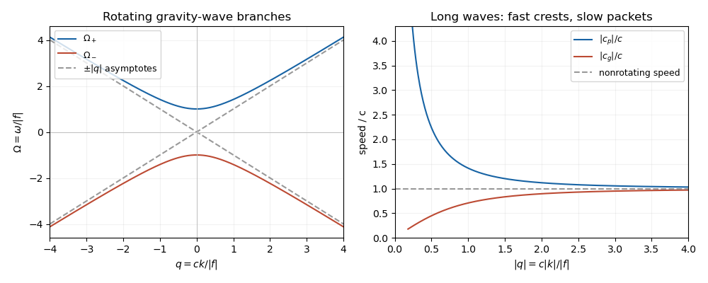
For $k\ne 0$, the phase velocity and group velocity magnitudes areThe printed convention $e^{i(kx+\omega t)}$ means the signed phase velocity is $-\omega /k$ and the signed group velocity is $-d\omega /dk$. The speed magnitudes above are independent of that sign convention.

For $f\ne 0$, longer wavelengths have greater phase velocity but smaller group velocity: individual crests and wave packets therefore answer “faster or slower” differently. At long wavelength, $|k|\ll |f|/c$, the frequency is nearly the inertial frequency $|f|$, $|c_p|\sim |f|/|k|$, and $|c_g|\sim c^2|k|/|f|$. Rotation has its largest relative effect here, and the waves are strongly dispersive. At short wavelength, $|k|\gg |f|/c$, both speeds tend to $c$ and rotation gives only a small, weakly dispersive correction. If $f=0$, the gravity waves are nondispersive, with speed $c$; at $k=0$ the phase velocity formula is undefined.

The Mészáros effect suppresses the growth of modes which enter the horizon during radiation domination. Modes with comoving wavenumber $k\gg k_{\mathrm{eq}}$ enter earlier, but gain only a logarithmic growth factor until matter-radiation equality; modes entering during matter domination grow as $a$ after entry. Consequently small-scale amplitudes are reduced relative to an extrapolation of the unsuppressed large-scale cosmological density power spectrum, creating a turnover near the matter-radiation equality scale $k_{\mathrm{eq}}={\mathcal{H}}_{\mathrm{eq}}$ in units $c=1$.

More quantitatively, for adiabatic primordial fluctuations with scalar spectral index $n_s$, the late-time linear spectrum can be written, up to a time-dependent normalization,The cold-dark-matter transfer function approaches a constant at $k\ll k_{\mathrm{eq}}$, whereas logarithmic small-scale matter transfer gives $T(k)\propto (k_{\mathrm{eq}}/k{)}^2\log (k/k_{\mathrm{eq}})$ at large $k$. ThusFor approximately scale-invariant initial curvature fluctuations, $n_s\simeq 1$, the large-$k$ scaling is $k^{-3}{\log }^{2}k$, rather than $k$. This discussion ignores baryonic acoustic structure and nonlinear clustering. The Mészáros equation solution basis includes both a constant and a logarithmic branch during radiation domination; the physical logarithmic growth is selected by matching the earlier radiation forcing, so not every mathematical solution grows logarithmically.

On a length scale $\ell$, pressure communicates support over a sound-crossing time $\ell /v_s$, whereas self-gravity acts over a time of order $(G{\rho }_0{)}^{-1/2}$. When the former is longer, gravity can amplify an overdensity before pressure smooths it. Thus Jeans instability occurs at scales of order $\ell \gtrsim v_s/\sqrt{G{\rho }_0}$; the precise numerical factor depends on whether scale means wavelength or inverse wavenumber.

Take a uniform static background, small perturbations, an inviscid barotropic fluid, and $\delta p=v_s^2\delta \rho$ with $v_s^2=(dp/d\rho {)}_0>0$. An infinite Newtonian homogeneous density cannot itself have zero background gravitational acceleration while satisfying the unmodified Poisson equation for Newtonian gravity. Specify the Jeans swindle: subtract the homogeneous field, or regard an external prescription as balancing it, and apply Poisson's equation only to perturbations. The linearized continuity equation and Euler equations for an inviscid fluid areTaking a time derivative of the first equation and substituting the second yields ${\partial }_t^2\delta \rho =v_s^2{\nabla }^2\delta \rho +4\pi G{\rho }_0\delta \rho$. A plane wave $e^{i(\mathbf{k}\cdot \mathbf{x}-\omega t)}$ therefore givesFor $0<k<k_J$ there is exponential growth at rate $\sqrt{4\pi G{\rho }_0-v_s^2{k}^2}$. At $k_J$ the density mode is neutral to this linear order, and above it there are acoustic oscillations. The critical wavelength is $2\pi /k_J=\sqrt{\pi }{v}_s/\sqrt{G{\rho }_0}$. Transverse velocity perturbations decouple as zero-frequency vortical modes in this idealization.

For the attractive Yukawa potential, assume a real screening parameter $\alpha \ge 0$. Its Green function obeys $({\nabla }^2-{\alpha }^2)(-Gm{e}^{-\alpha r}/r)=4\pi Gm{\delta }^{(3)}(\mathbf{r})$, including the delta source. Thus $\delta {\varphi }_{\mathbf{k}}=-4\pi G\delta {\rho }_{\mathbf{k}}/(k^2+{\alpha }^2)$. The same fluid elimination gives Jeans instability with Yukawa gravity:There exists a growing nonzero-wavenumber mode precisely whenEquality gives no exponentially growing nonzero mode. If screening exceeds this threshold, the finite-range gravitational response is too weak to overcome pressure at any wavelength. Otherwise all sufficiently long but nonconstant waves remain unstable, with a longer minimum unstable wavelength than in Newtonian gravity. For $\alpha >0$ the long-wave gravitational contribution also scales as $k^2$, so the growth rate tends to zero as $k\to 0$; screening does not produce a second positive lower cutoff in wavenumber. A homogeneous screened background can have the constant gravitational potential $-4\pi G{\rho }_0/{\alpha }^2$, with zero force, so no Newtonian background subtraction is needed for nonzero screening. The limits $k\to 0$ and $\alpha \to 0$ are nonuniform. An exact $k=0$ density change is not one of the growing finite-wavelength modes. In the pressureless edge case $v_s=0$, every finite $k>0$ is unstable for positive density and finite screening.

Separate the uniform stream and an arbitrary time-dependent gauge from each velocity potential: ${\varphi }_j=U_{j}x+f_j(t)+{\varphi }_j^{\prime }$. Only gradients of the velocity potential determine the velocity field. The remote fluid must remain in its unperturbed uniform stream, soAfter fixing the harmless gauge, the nonzero-wavenumber perturbation velocity potentials themselves vanish at the corresponding infinities. Incompressible flow and irrotational flow give the Laplace equation for each perturbation. For a normal mode with $k>0$, the vertical amplitude solves ${\Phi }_j^{\prime \prime }-k^2{\Phi }_j=0$, henceThe opposite exponentials are excluded because they make the perturbation grow at infinity. It is the perturbation, rather than the total potential $U_{j}x+f_j(t)$, that decays.

For an odd velocity potential, chooseAt $z=L$ the two kinematic conditions give $A=ic{B}_{+}$ and $C\cosh (kL)=i(V-c)B_{+}$. The dynamic condition is $-cA=(V-c)C\sinh (kL)$. Eliminating $A,C,B_{+}$ gives, with $s=\tanh (kL)$,The lower interface gives the same equation by odd parity of the velocity potential. The interior vertical velocity is even, so $B_{-}=B_{+}$: the displacement is a sinuous mode of a planar jet even though the potential is odd.

For $L>0$, $V\ne 0$ and $k>0$, $0<s<1$ and one root has $c_i>0$. Thus every nonzero wavenumber is unstable in this ideal top-hat planar jet. The phrase “all choices” is understood with these assumptions: $k=0$ has no exponential wave growth, and $V=0$ has no shear.

At the absolute wavenumber, the group velocity $d\omega /dk$ is zero. The corresponding accessible saddle therefore governs the disturbance seen at a fixed position. Its exponential growth rate isSaddle accessibility can be checked directly here. With $D=1+i{c}_d$, whose real part is positive, Fourier inversion gives the Green function of the linear complex Ginzburg-Landau equation,At fixed $x$ its exponential rate is $\mathrm{Im}{\omega }_0$, while along the packet centre $x=Ut$ it is $\mu$. For real wavenumbers of Fourier modes, the temporal growth rate is $\mathrm{Im}\omega (k)=\mu -k^2$, so the flow is temporally unstable exactly when $\mu >0$.

Consequently the classifications for a localized disturbance in this laboratory frame areFor convective hydrodynamic instability, a travelling wave packet amplifies but the response at each fixed position decays. For absolute hydrodynamic instability, that fixed-position response amplifies. The equality is the marginal absolute threshold: its exponential rate is zero and the impulse response has a $t^{-1/2}$ prefactor. For $\mu <0$ there is no temporal growth; $\mu =0$ is temporally marginal. When $U=0$ the convective window is empty. These conclusions use the infinite-line impulse problem; a general dispersion relation requires its own spatial-branch or saddle selection.

Take the physical coefficients $U,\mu ,c_d$ real. Substitution of $e^{i(kx-\omega t)}$ into the linear complex Ginzburg-Landau equation gives $-i\omega +ikU-\mu +(1+i{c}_d)k^2=0$, henceLet $A=c_d-i$. Completing the square yields $\omega =A(k+U/(2A){)}^2+i\mu -U^2/(4A)$. Therefore the absolute wavenumber and absolute frequency areTheir explicitly separated parts areThus $d\omega /dk=U+2(c_d-i)k$ vanishes at $k_0$. The complex saddle describes the localized Green function response; it is different from selecting a real wavenumber for a Fourier mode for temporal amplification.

When $R\ll Q$, the ratio of cubic damping to linear amplification is $R^2/Q^2\ll 1$. The cubic amplitude saturation equation therefore giveswhile the small-amplitude regime lasts. With $c_d=0$, the matching real-wavenumber normal mode of the linear complex Ginzburg-Landau equation has $\omega =Uk+i(\mu -k^2)$ and hence amplitude proportional to $e^{(\mu -k^2)t}$. ThusThis is the temporal growth rate of the same Fourier component. It is not the fixed-position absolute frequency rate $\mu -U^2/4$ of a localized impulse. Nonlinear damping becomes important when $R$ is comparable with $Q$ and then arrests exponential amplification.

Take $z$ upwards and write $\zeta =z+Wt$, so that the unperturbed interface is $\zeta =0$, with carbon dioxide above and water below. Use the sharp-interface, incompressible flow version of Darcy's law, with constant porosity and permeability of a porous medium, no capillary pressure, and effectively unbounded layers. The distinction between Darcy flux and interface speed matters: the base flux is $q_z=-\varphi W$, since the printed $W$ is the speed of the interface. Thus the base pressure gradients satisfyThe mass density ordering is stabilizing, whereas injection of the less viscous fluid into the more viscous fluid produces the Saffman–Taylor instability.

For linear stability analysis, displace the interface by $\eta =\hat{\eta }{e}^{\sigma t+i\alpha x}$. Taking the divergence of Darcy's law shows that the perturbation pressure satisfies the Laplace equation. Decay away from the interface gives, for $a_{\alpha }=|\alpha |>0$,The kinematic boundary condition and continuity of normal Darcy flux giveMeanwhile pressure continuity, evaluated on the displaced interface, givesEliminating $A,B$ yields the buoyancy-modified Darcy fingering dispersion relation:Every nonzero wavenumber decays when $W<W_c$, grows when $W>W_c$, and is neutral at equality, whereThe zero wavenumber is a uniform displacement and is neutral. Without a short-scale regularization such as surface tension, this model has no fastest-growing finite wavenumber: on the unstable side its growth rate increases without bound as $|\alpha |$ increases. Finite layer depths would change the dispersion relation; none are specified here.