The third-order correlation width of a Gaussian pulse converts a measured ideal third-order intensity autocorrelation width to the width of its assumed Gaussian intensity profile. If the pulse intensity has temporal standard deviation ${\sigma }_I$, its squared intensity gate has deviation ${\sigma }_I/\sqrt{2}$. Their cross-correlation haswhere both $\tau$ values are intensity full widths at half maximum. The parent third-order intensity autocorrelation article derives the complete Gaussian trace by integration. The factor concerns that shape family and that correlation definition; it is not a universal pulse-width conversion.

A focused extension separates a known instrument response. Suppose an additional normalized Gaussian response of width ${\tau }_R$ convolves the ideal trace. Addition of Gaussian variances givesFor an original chosen ${\tau }_{\mathrm{measured}}=120\mathrm{fs}$ and ${\tau }_R=60\mathrm{fs}$, the inferred pulse width is $84.9\mathrm{fs}$. Applying only the ideal conversion would give $98.0\mathrm{fs}$. This Gaussian instrument broadening in third-order pulse correlation assumes that the additional response really acts as a Gaussian convolution; it is not an empirical correction for every correlator.

The historical physical implementation used second-harmonic generation followed by sum-frequency generation and spatial delay encoding.^[ref] Optical gate width, phase matching and spatial overlap belong to its response model. A finer scan step alone does not demonstrate a smaller optical response width.

If the assumed response width equals or exceeds the measured width, the displayed subtraction does not provide a resolved positive pulse width. Non-Gaussian traces, satellites and chirped fields also require explicit modeling; an intensity-width conversion does not reconstruct the optical wave phase.

The haline contraction coefficient measures the fractional increase of mass density with salinity at fixed temperature and pressure:Its units depend on the salinity variable $S$: a dimensionless mass fraction and a value in grams per kilogram require different numerical coefficients.

For small changes, $\delta \rho /\rho \simeq -\alpha \delta T+\beta \delta S$, with thermal expansion coefficient $\alpha$. This formula separates two competing buoyancy contributions. In thermosolutal convection, their combination determines the static density gradient, while unequal diffusion rates determine whether that apparently stable gradient can nevertheless become unstable.

In double-diffusive convection, a density ratio compares the buoyancy contributions from two stratifying quantities. A convention must be stated. For vertical coordinate $z$ increasing upward and warm salty water above cooler fresher water, take $R_{\rho }=\alpha T_z/(\beta S_z)$, with positive thermal expansion coefficient $\alpha$ and haline contraction coefficient $\beta$.

The linear equation of state gives ${\rho }_z={\rho }_0(-\alpha T_z+\beta S_z)$. Thus $R_{\rho }>1$ makes the combined density stratification stable, even though the salt contribution alone is destabilizing. Faster heat diffusion can still enable salt fingering. The reciprocal ratio is also used in the literature, so a numerical density ratio is meaningless without its convention.^[ref]

Over $\mathbb{C}$, the border rank of a tensor $T$ is the least $r$ for which $T$ lies in the closure of tensors of tensor rank at most $r$. The usual Euclidean topology and Zariski topology give the same closure here. Hence $\underline{R}(T)\le R(T)$, but equality need not hold.^[ref]

Let $e_0,e_1$ be a basis of ${\mathbb{C}}^2$ and putFor nonzero $\epsilon$,Each approximant is a sum of two pure tensors, so the border rank is at most two. It is not one, since a matrix obtained by separating one factor from the other two has rank two.

Its exact tensor rank is three. The two tensor slices in the first factor span $\left\{\left(\begin{array}{cc}b& a\\ a& 0\end{array}\right):a,b\in \mathbb{C}\right\}$. Its determinant is $-a^2$, so this space has only one rank-one direction. A rank-two tensor with two independent slices would require their span to be generated by two independent rank-one matrices, a contradiction. The limit therefore permits a decomposition that is impossible exactly.

A bilinear algorithm computes a bilinear map $b:U\times V\to W$ by multiplying linear expressions in the two inputs and linearly combining the results. A length-$r$ algorithm has the formwith ${\alpha }_j\in U^{\ast }$, ${\beta }_j\in V^{\ast }$ and $w_j\in W$. Its multiplication count is the number of products between input-dependent expressions; additions and multiplication by fixed constants are accounted for separately. The smallest possible length is the tensor rank of the associated tensor in $U^{\ast }\otimes V^{\ast }\otimes W$.^[ref]

For multiplication of complex numbers over the real numbers, the usual formulas use four real products. Instead compute $p=ac$, $q=bd$ and $r=(a+b)(c+d)$. ThenOnly three real products are needed. This saves a multiplication by sharing intermediate information between the two outputs.

The coefficient field and cost model matter. Allowing divisions by expressions depending on the input is outside this bilinear model. Border rank also allows limits of algorithms and can be smaller than the minimum length of an exact bilinear algorithm.

Bounding uncollected expiratory volume from terminal flow uses an explicit restriction on future volumetric flow rate to limit the air missed when a recorded expiration stops. A small final volumetric flow rate alone gives no such guarantee: an arbitrarily long, slowly decaying tail can have substantial remaining volume.

Let $q(s)$ be the nonnegative future volumetric flow rate, with $s=0$ at the recording endpoint. Suppose an independently justified bound on its decay holds throughout the tail:Differentiating $e^{s/{\tau }_{\max }}q(s)$ shows that it cannot increase. HenceThis is an upper bound from a specified differential inequality, not a fitted exponential silently treated as established physiology.

For original values $q_T=0.04\mathrm{L}{\mathrm{s}}^{-1}$ and ${\tau }_{\max }=3$ s, the missed volume is at most 0.12 L. If the collected volume is $M=3.00$ L and the correctly captured first-second volume is $A=2.40$ L, thenIf the terminal instrument reading has a deterministic error bound $u$, use $q_T\le q_{\mathrm{measured}}+u$ in the same argument. An uncertainty statement about the final reading does not itself establish the future decay assumption.

The assumption is essential. Exponential tails $q(s)=q_T{e}^{-s/\tau }$ with the same terminal volumetric flow rate have missed volumes $q_T\tau$, unbounded as $\tau$ increases. This explains why the endpoint of a trace cannot by itself certify complete expiration. The primary spirometry statement separately specifies end-of-forced-expiration and measurement acceptability criteria.^[ref] The inequality is an illustrative model bound, not an additional clinical stopping rule.

The standard symplectic plane is ${\mathbb{R}}^2$ with the closed nondegenerate two-form $\omega =dq\wedge dp$. For tangent vectors $u=(a,b)$ and $v=(c,d)$,their signed parallelogram area. This alternating pairing is not a positive-definite inner product: every vector pairs to zero with itself.

A linear map $A$ preserves the form exactly when $\det A=1$, because $\omega (Au,Av)=\det (A)\omega (u,v)$. Thus $\mathrm{Sp}(2,\mathbb{R})={\mathrm{SL}}_2(\mathbb{R})$. A nonlinear example is the shear $(q,p)\mapsto (q,p+q^2)$, whose pullback form is $dq\wedge (dp+2qdq)=dq\wedge dp$.

Every smooth embedded curve in the plane is Lagrangian: the restricted two-form vanishes on its one-dimensional tangent spaces, which have half the ambient dimension. The symplectic plane is therefore the simplest model of symplectic area preservation and Lagrangian geometry.

Recurrent postoperative event analysis studies several qualifying events occurring in the same patient after surgery, rather than retaining only a first event or the highest severity grade. It requires an event definition that distinguishes a new episode from another observation of an ongoing episode. The original Clavien-Dindo classification validation deliberately registered the most severe complication for patients with several; a recurrent-event question requires more of the event history.^[ref]

Let $N_i(t)$ count qualifying events in patient $i$ by postoperative time $t$. This is a counting process. With complete observation of $n$ independent patients through $t$, the mean cumulative postoperative event count has the simple estimatorIt describes average accumulated burden. It is different from the probability $\mathrm{Pr}(N_i(t)\ge 1)$ of any event, and neither quantity specifies the severity of the events counted.

Within-patient dependence matters for uncertainty. At a fixed time, write $K_i=N_i(t)$ and let $s_K^2$ be the usual sample variance across patients. The patient-based standard error of the mean is $s_K/\sqrt{n}$ under independent-patient sampling. An original four-patient illustration with counts $(0,0,0,4)$ gives mean $1$, sample variance $4$ and estimated standard error $1$. Treating the total count as a Poisson count would instead give $\sqrt{4}/4=0.5$. This small example demonstrates different model assumptions; it does not validate either model or a normal confidence interval for four patients.

A proper record includes patient identity, episode times, resolution rules, severity and observation periods. Resampling patients with all their events intact can preserve within-patient dependence; resampling individual events as though they came from unrelated people cannot. An event intensity model may additionally condition on previous events, evolving health and exposure time, rather than assuming a constant rate.

Incomplete follow-up and death change the question. A rate among people currently alive and observed differs from total expected burden per original operated patient. Death prevents future postoperative events, whereas loss to follow-up hides whether events occurred. These require explicit observation and competing risks assumptions instead of an automatic independent-censoring treatment. The scientific aim is to measure repeated burden without confusing events, patients and time at risk.

Cassiopeia A is a young Galactic supernova remnant, containing expanding stellar debris, shock-heated gas and a compact central object. Observations at different wavelengths reveal different physical components rather than interchangeable pictures of the same emission process.

X-rays trace very hot material and elemental signatures, while infrared observations can reveal cooler dust and gas. Comparing spatial distributions and velocities helps reconstruct how the star exploded and how its ejecta interact with surrounding material.^[ref]

For a finite-valued subordinator $T$ starting at zero, the Laplace exponent of a subordinator is the function $\Phi$ determined byIts Lévy–Khintchine formula takes the formwhere $d$ is the deterministic drift coefficient and $\nu$ is the Lévy measure. This representation separates steady motion of the clock from its positive jumps.^[ref]

For a deterministic clock $T_t=dt$, $\Phi (\lambda )=d\lambda$. For a Poisson process of rate $a$ with unit jumps, $\Phi (\lambda )=a(1-e^{-\lambda })$. For a sum of independent subordinators, the Laplace exponent of a subordinator is the sum of the individual functions, because the Laplace transforms multiply. The transform at $\lambda =0$ gives $\Phi (0)=0$.

A coverage function assigns a value to the union of objects covered by a selection. Let $V$ index sets $C_v$ in a finite universe $U$. The unweighted version isA weighted coverage function gives each $u\in U$ a nonnegative weight $w_u$ and sums those weights over the same set union. Its value is zero on the empty selection and cannot decrease when more sets are selected.^[ref]

The submodular set function property follows from an explicit marginal calculation:If $S\subseteq T$, the objects still uncovered after $T$ form a subset of those uncovered after $S$. Nonnegative weights therefore make the gain no larger after $T$: precisely the diminishing returns property.

For an original example, take $C_1=\{a,b\}$, $C_2=\{b,c\}$ and weights $(w_a,w_b,w_c)=(2,1,3)$. Then $F(\{1\})=3$, $F(\{2\})=4$ and $F(\{1,2\})=6$. The second set adds only three after the first, because their shared object $b$ is counted once. This models the value of distinct coverage, rather than the sum of overlapping collection sizes.

For a set function $F:2^{\{1,\dots ,n\}}\to \mathbb{R}$ with $F(\varnothing )=0$, sort the coordinates of $x\in {\mathbb{R}}^n$ as $x_{{\pi }_1}\ge \cdots \ge x_{{\pi }_n}$, and put $S_k=\{{\pi }_1,\dots ,{\pi }_k\}$. The Lovász extension isTies do not affect the result, because equal-coordinate terms telescope. At an indicator vector $1_S$ it gives $f(1_S)=F(S)$, so it extends a discrete objective to a piecewise linear function on a vector space.

For $F(S)=1$ when $S\ne \varnothing$ and zero otherwise, $f(x)={\max }_i{x}_i$. More generally, the extension is a convex function exactly when $F$ is a submodular set function. This equivalence is what makes the construction useful: a diminishing-returns condition on subsets becomes a geometric property on real vectors.^[ref]

The standard basis vector $e_i$ in ${\mathbb{F}}^n$ has coordinate one in position $i$ and zero elsewhere. Every vector $v=(v_1,\dots ,v_n)$ has the unique expansion $v={\sum }_{i=1}^n{v}_i{e}_i$.

For example, $e_2=(0,1,0{)}^{\top }$ in three dimensions. The outer product $e_i{e}_j^{\top }$ is the matrix unit with a single one in row $i$, column $j$, providing a standard basis for matrices as well. The word standard refers to the chosen coordinate representation; an abstract vector space does not come with a distinguished coordinate basis automatically.

Co-oximetry determines hemoglobin composition using optical measurements at multiple wavelengths. In a laboratory blood analyzer, it can distinguish oxyhemoglobin, deoxyhemoglobin, carboxyhemoglobin and methemoglobin rather than infer all hemoglobin behavior from a single oxygen-related number. A manufacturer description explicitly identifies direct optical spectrophotometry as the measurement method for its analyzer's co-oximetry parameters.^[ref]

An idealized mixture model makes the separating information explicit:where $A_j$ is measured absorbance, $\ell$ the path length, $c_i$ a species concentration, ${\epsilon }_i$ its molar absorption coefficient and $b_j$ a background term. Estimating four unconstrained concentrations requires sufficient independent spectral observations and known response coefficients; merely having four wavelength labels does not guarantee independence. An isosbestic point shared by two species supplies information about their combined amount but cannot by itself separate their proportions.

The denominator of a reported fraction matters. In a simplified four-form example, stipulate $90\%$ oxyhemoglobin, $5\%$ deoxyhemoglobin, $4\%$ carboxyhemoglobin and $1\%$ methemoglobin, all expressed on the same total-hemoglobin basis. Fractional oxyhemoglobin is $0.90$, but the functional oxygen saturation isThese differ because the second denominator excludes the other two forms. The manufacturer's parameter description distinguishes these definitions.^[ref] The chosen fractions are an explanatory example, not clinical thresholds.

A blood-sample optical assay and a noninvasive pulsatile optical measurement use different observation models. Their output labels and denominators must be established from the specific method, rather than inferred from the common word oximetry. Likewise, oxygen partial pressure describes dissolved oxygen equilibrium and is not itself a measurement of all hemoglobin fractions.

An instrument test can compare reference mixtures with independently established composition, record full spectral residuals and vary a suspected interferent. Agreement of one derived saturation number alone does not validate every inferred species concentration. Background, spectral overlap and sample handling belong in the measurement model and its uncertainty.

Offset sensitivity of log-ratio nail models describes the bias produced when an additive background enters a ratio used to estimate a nail plate parameter. A shared multiplicative gain cancels from an ideal ratio, whereas a shared additive term generally remains.

Consider the original simplified spectral model $y_j=r{e}^{-2{\mu }_{j}h}$, with plate thickness $h$, known attenuation coefficients ${\mu }_j$ and wavelength-independent effective reflectance $r$. Write $\Delta \mu ={\mu }_1-{\mu }_2\ne 0$. The ideal thickness is $h=\log (y_2/y_1)/(2\Delta \mu )$. If measured signals are $s_j=g{y}_j+b$ with $g>0$, define the input-equivalent offset $\beta =b/g$. Ignoring that offset givesBoth offset-adjusted signals must be positive. Equal additive errors do not cancel inside this logarithm.

With stipulated $r=0.8$, $h=0.5$ mm, ${\mu }_1=1\mathrm{m}{\mathrm{m}}^{-1}$ and ${\mu }_2=0.5\mathrm{m}{\mathrm{m}}^{-1}$, the signals are about 0.2943 and 0.4852. Adding $\beta =0.020$ gives an apparent thickness of about 0.4746 mm. Positive background pulls the ratio towards one and underestimates thickness in this example. The numbers are model calculations, not an experimentally validated nail-thickness calibration.

The local sensitivity isAt zero offset in the example it is approximately $-1.337\mathrm{mm}$ per unit normalized signal. A residual-offset standard uncertainty of 0.005 therefore contributes approximately 0.00668 mm to the local thickness uncertainty. If that same uncertain background correction is reused across channels, its errors are correlated; the covariance terms belong in the propagation model.^[ref]

Residual-offset uncertainty in nail thickness estimates remains even when repeated photon measurements reduce random fluctuations. A useful test measures dark current and examines optical background separately, since fluorescence need not have the same spectral dependence as either. The primary nail-transmission study explicitly included a fluorescence correction.^[ref] That motivates identifying the background component; it does not validate this reduced thickness model.

Scaled subtraction of two spatially offset Raman spectra suppresses a common surface contribution by matching its amplitude between two measurements. The spatially offset Raman spectroscopy experiment establishes that collection offset can change surface and buried-layer proportions; numerical separation then needs a model of those contributions.^[ref] The following two-component subtraction is an original simplified case, not a claim that it reproduces the paper's full analysis.

Let fixed Raman spectra $S(\nu )$ and $B(\nu )$ describe the surface and buried material. Writewith $a_0\ne 0$. ThenIf the two mixing proportions are identical, so $a_0{b}_1-a_1{b}_0=0$, this cancels the buried component too. Offset diversity must supply different mixtures, not merely a weaker copy of the same spectrum.

For an original example, take $Y_0=10S+B$ and $Y_1=4S+3B$. The correct scale $k=0.40$ gives $Z=2.6B$. Using $k=0.42$ instead gives $Z=-0.2S+2.58B$: an incorrectly subtracted surface band can produce a negative residual even when both true spectra are nonnegative. A surface-specific reference band can estimate the scale only if the assumed common shape and response are adequate.

Noise remaining after scaled Raman subtraction is distinct from the cancelled mean signal. At a surface-only channel, suppose two independent acquisitions have Poisson photoelectron counts with means $10000$ and $4000$. For fixed $k=0.40$, the expected residual is zero, butgiving a standard deviation of about $74.8$ in the scaled count units. Subtraction has not erased shot noise. Correlated acquisitions and uncertainty in $k$ add further terms. Varying shape, wavelength-dependent attenuation or an unmatched fluorescence background can invalidate this simple linear separation.

Mass-normalized temporal kernels for nail clippings assign each earlier material time its fraction of the analyzed sample's mass. They convert a finite clipping into an averaging operator on a time-dependent retained concentration. The weighting is normalized by the assayed material amount, rather than by elapsed time alone.

For an original one-dimensional advection model, let $s$ be the time when a material element crossed a defined anatomical reference, and collect at time $t$. With spatially uniform positive advance speed $v(u)$,Suppose the clipping's retained elements correspond to $s\in [s_1,s_2]$. Let $m(x,t)$ be structural mass per unit length at collection, and assume the marker's concentration per structural mass is preserved along each element. ThenThe kernel has units of inverse time, is nonnegative and integrates to one. It can be treated mathematically like a probability density function for the reference-crossing time of material selected in proportion to its mass. This is a material-accounting interpretation, not a claim that the biological transport is random.

For a stipulated 20-day window, take line density 1 mg/mm, advance 0.10 mm/day in the earlier ten days and 0.20 mm/day in the recent ten days. The two intervals contribute 1 and 2 mg, respectively. Their kernel heights are $1/30$ and $1/15$ per day. A retained concentration of 90 ng/mg only in the earlier interval gives $\overline{c}=30$ ng/mg; a uniform time average would give 45. A constant 30 ng/mg history gives the same sample result. Thus one pooled measurement does not identify a unique history.

A centroid date of a mass-normalized nail kernel summarizes the weighting, while the kernel's spread records its finite time resolution. Neither removes the difference between reference crossing and earlier formation in the hidden nail matrix. The primary nail-marking experiment measures displacement over observation intervals, not the complete kernel or marker retention law.^[ref] Measuring segment mass, geometry and growth history constrains separate parts of this model.

A pressure-tap spatial footprint describes the finite region of a surface pressure field that contributes to a tap's response, rather than treating the reading as an exact point value. A pressure-footprint response kernel can represent spatial averaging in a simplified linear model. A real opening can also disturb the flow, so averaging is not a complete physical correction model.

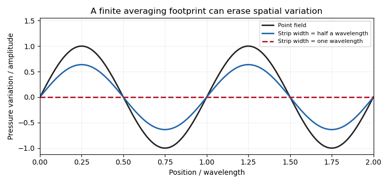
For an ideal one-dimensional strip of width $w$, suppose the reading at $x_0$ isFor a smooth field, a Taylor expansion gives $p_m=p(x_0)+p^{\prime \prime }(x_0)w^2/24+O(w^4)$. Symmetry cancels the first-order gradient term, but not curvature. For an exactly quadratic field this expression through $w^2$ is exact. It shows why a footprint cannot in general be summarized by a displaced point location.

If $p(x)=A\sin (kx)$, direct integration instead givesThe multiplier is a sinc function. For wavelength $\lambda =2\pi /k$, a half-wavelength strip retains $2/\pi \approx 0.637$ of the amplitude, while a full-wavelength strip gives zero. These results concern an ideal strip spatial averaging filter, not an asserted weighting law for a circular pressure hole.

An actual wind tunnel experiment by E. B. Plentovich and Blair B. Gloss used interchangeable orifices in a flat plate. Increasing opening size increased the observed pressure error; a flush porous-metal plug reduced it under the tested conditions.^[ref] This is direct evidence that opening geometry affects the measurement, including through local flow disturbance.

Footprint characterization and tap spacing address separate limitations. Closely spaced readings from broad footprints may still suppress short spatial variations, while narrow footprints sampled too sparsely can suffer spatial aliasing. Neither problem is removed merely by improving the precision of the pressure transducer.

Elliptic span loading is a distribution of lift per unit span proportional to a half-ellipse, vanishing at both tips of a planar wing. For span $b$ and total lift $L$, writeThe normalization follows by setting $s=2y/b$ and using ${\int }_{-1}^1\sqrt{1-s^2}ds=\pi /2$. It specifies a load distribution, rather than the wing outline. Classical lifting-line theory identifies this loading as the minimum-induced-drag solution for fixed total lift and span in its ideal planar setting.^[ref]

The loading corresponds to circulation magnitude $\Gamma (y)={\Gamma }_0\sqrt{1-(2y/b{)}^2}$, with $L^{\prime }(y)=\rho U\Gamma (y)$ under the chosen positive-lift convention. Its ideal downwash at the lifting line is constant,Using dynamic pressure $q=\rho U^2/2$ recovers $D_i=L^2/(\pi q{b}^2)$ and the span efficiency factor $e=1$ in that normalization.

A Fourier series makes the minimum transparent. In the classical lifting-line expansion, put $y=(b/2)\cos \vartheta$ andAt fixed $C_L$ and $AR$, $A_1$ is fixed and every higher-order contribution to drag is nonnegative. The minimum has only $A_1$, yielding the half-ellipse. A higher-harmonic penalty in span loading quantifies departure from it: if $A_3=0.1A_1$ is the only additional term, $1/e=1+3(0.1{)}^2=1.03$, so $e\approx 0.971$ and induced drag rises three percent under the stated constraints.

For an original loading example, $L=6000\mathrm{N}$ and $b=10\mathrm{m}$ give a central load $763.94N/m$. At $y=b/4$ it is $0.8660$ of the central value. With $\rho =1.2kg/{\mathrm{m}}^3$ and $U=50m/s$, the model gives ${\Gamma }_0\approx 12.732{\mathrm{m}}^2/s$, $w\approx 0.6366m/s$ and $D_i\approx 76.39\mathrm{N}$.

A proposed test integrates measured surface pressure around several wing sections to estimate $L^{\prime }(y)$, then compares the normalized distribution and a wake survey with the model. An elliptic planform does not alone guarantee elliptic loading: section characteristics, incidence variation, deformation and operating conditions also enter. Nonplanar lifting systems, fixed bending-moment constraints and viscous or compressible effects change the optimization problem; the fixed-lift, fixed-span planar result should not be generalized beyond its assumptions.

The solar neutrino problem was the historical deficit of detected electron neutrinos relative to predictions based on solar fusion and detector response. The key ambiguity was whether the Sun emitted fewer neutrinos than expected or whether neutrinos changed flavor before reaching the detector.

The Sudbury Neutrino Observatory compared charged-current reactions sensitive primarily to electron neutrinos with neutral-current reactions sensitive to all active flavors. The electron-flavor flux was suppressed while a substantial non-electron active component was present, supporting flavor transformation rather than simply lowering the total solar production. Comparing channels therefore tested particle behavior independently of relying on one detector's count deficit.^[ref]