Topics (384k) Articles (398k) Users (410) Discussions (242) Comments (383) Files (13k) New article

Heat release rate is the rate at which a process releases energy as heat, commonly used to characterize combustion. It has the dimensions of power and is measured in watts, with . Using for cumulative released energy,The heat release rate is the height of the curve; total released energy is its area.
For a synthetic fire whose heat release rate rises linearly from zero to in and falls linearly to zero over the next , the area is a triangle:A second fire with a smaller peak but longer duration can release more total energy. A peak value alone therefore cannot describe the full event.
A fuel-based estimate multiplies fuel mass flow rate by the effective released energy per unit mass, under stated assumptions about composition and combustion. For a deliberately stipulated effective value and fuel rate , the estimate is . In oxygen consumption calorimetry, measured gas flow and oxygen depletion instead provide an estimate of heat release rate. NIST uses independently metered reference burners to compare these two inference routes.[ref]
Natural Gas Confirmation Burner by NIST. Research Overview, fuel-consumption heat input and confirmation of oxygen-consumption calorimetry
A fire's heat release rate differs from the heat transfer received by one nearby surface or from the temperature of its exhaust. Released energy can leave by several paths, while a receiving object can store internal energy as well as lose heat. Even a gas-based calorimeter needs a defined measurement boundary, capture conditions and time response. The NIST National Fire Research Laboratory provides an example of using exhaust collection to quantify large-fire heat release rate.[ref]
National Fire Research Laboratory by NIST. Facility description, large-fire calorimetry and exhaust systems
A torus-fixed point of a toric variety is a point left unchanged by every element of its acting algebraic torus. In a normal split toric variety of dimension , the orbit-cone correspondence givesConsequently fixed points correspond exactly to full-dimensional cones. Maximality under containment is not enough if a maximal cone has smaller dimension.
For with coordinatewise scaling, the origin is fixed. Points on a punctured coordinate axis have one-dimensional orbits, while points with both coordinates nonzero lie in the dense two-dimensional orbit. For the positive-dimensional torus itself, multiplication has no fixed point.
The fan consisting only of the two positive coordinate rays and zero describes . Both rays are maximal cones, but neither is full-dimensional, so there are no fixed points. This example isolates the dimension condition from the informal idea of a maximal face.[ref]
A time-changed filtration records the information available after a new clock has reached an old time. Let be a filtration and let be a nondecreasing family of finite stopping times. DefineThe second expression is the stopping-time sigma-algebra. If and , thenThus , as required for a filtration.
For the deterministic clock , the new information is , not . A continuous adapted process sampled at these stopping times is adapted to the new filtration. Preservation of the local martingale property requires further hypotheses such as those in the optional time-change theorem; merely substituting arbitrary random times does not establish it.
A momentum buffer stores an accumulated history of gradients for an optimization algorithm. In one common convention, a parameter vector , supplied gradient , learning rate and constant coefficient obey the recurrence relationThe buffer belongs to the optimizer state: it remembers earlier inputs even when the current parameters are unchanged. This is the undampened momentum convention used by PyTorch stochastic gradient descent with weight decay and the Nesterov accelerated gradient method disabled; its documented first buffer is the first gradient, agreeing with this recurrence from . Other conventions absorb the learning rate into the stored buffer, so a buffer value needs its update convention to be interpreted.[ref]
SGD in the PyTorch documentation. PyTorch2.15, algorithm and note comparing momentum conventions and first-step initialization
Repeated substitution gives the exponentially weighted gradient historyTo verify this identity, substitute its expression for into : multiplication by raises every old exponent by one, and the added is precisely the new exponent-zero term. The formula holds at because its sum is empty, completing the mathematical induction.
For an original scalar example with and a constant supplied gradient , the geometric series yields . At , and the limit is 10. The buffer is an unnormalized sum: multiplying it by changes its scale, and would require a corresponding learning rate adjustment to preserve these parameter updates.
The same memory explains why momentum can temporarily oppose the current gradient. If , and the new scalar gradient is , then . With a positive learning rate, the parameter still decreases, although the present negative gradient alone would call for an increase. Persistence can carry motion through rapidly alternating gradients, but this example also shows why the rule need not decrease the objective function at every step.
An optimization checkpoint is a saved description of an ongoing optimization algorithm from which its optimizer updates can resume. It combines the current parameters with the relevant optimizer state. The practical criterion is optimizer restart equivalence: after restoring the saved information and supplying the same subsequent inputs, the chosen update rule should produce the same subsequent states.
For a deterministic scalar example, minimize the quadratic function with gradient , learning rate and momentum buffer recurrence , followed by . Start with . After one step the saved pair is . Restoring both gives and . Restoring only and initializing a new momentum buffer to zero gives and . Equal saved parameters can therefore lead to unequal continuations. These numbers are an original calculation for the declared recurrence.
In PyTorch, a general training checkpoint commonly serializes separate model and optimizer dictionaries, together with the training position. The model dictionary contains learned parameters and registered model buffers; the optimizer dictionary contains its own changing state and group settings.[ref]
Saving and Loading Models in the PyTorch tutorials. What is a state_dict?; Saving & Loading a General Checkpoint for Inference and/or Resuming Training
Restoring the optimizer state-to-parameter association also matters: the optimizer loader pairs stored identifiers with parameters in group order, without independently establishing that they denote the same mathematical parameters.[ref]torch.optim in the PyTorch documentation. PyTorch2.15, Optimizer.state_dict, state/param_groups and loading note
The required checkpoint boundary depends on the computation being resumed. A changing learning rate schedule, the next position in the training data, and the state of a pseudorandom number generator can influence future updates. Matching them is part of computational reproducibility; a saved parameter vector alone does not specify the whole training process.
Optical contrast in decibels expresses a specified ratio logarithmically. For peak-to-local radiant power contrast ,The inverse convention gives . State the convention and the time of the weak feature. A peak-to-feature contrast means one million to one in power, not in field amplitude.
An original readout example uses a linear photodetector whose baseline-corrected output is proportional to optical power. A main reading of and weak-feature reading of imply and . Applying to those readings would incorrectly report : the electrical signal represents power, not optical wave amplitude.
If instead a measurement is proportional to an optical field amplitude , with the same impedance and spatial normalization for both fields, power is proportional to . ThenA field-amplitude ratio of and a power ratio of therefore express the same contrast. The correct multiplier follows the measurement model, not whether the readout unit happens to be volts.
Contrast does not specify pedestal energy fraction, optical prepulse duration or delay coverage. The Sequoia primary sheet specifies dynamic range, scan range and optical temporal resolution separately.[ref]
Sequoia temporal contrast measurement by Amplitude. January2024 technical sheet, PDFp2, Specifications
A signal beneath a known measurement floor supports a contrast bound within that window; subtracting an uncertain background does not establish unlimited contrast.In online learning, cumulative regret compares the total loss of sequential choices with the best fixed action that could have been chosen in hindsight:The comparator uses one action for every round; comparing with a different best action at each round defines a stronger benchmark. For two actions whose losses over three rounds are and , always choosing the second has loss two, while the best fixed action has loss one, giving regret one.
A bound means average regret tends to zero. It does not promise zero loss or identify a true data-generating probability distribution; even adversarial loss sequences can be studied this way. In a multi-armed bandit, only the chosen action's reward is observed, making information gathering part of the decision problem.
Finite-time ambiguity between stiffness and slow filling means that a small volume response at one time can come from a stiff compartment or from a more compliant compartment that has not finished filling. In a passive single-compartment pressure-step model,One observation supplies one equation for equilibrium lung compliance and time constant . It does not generally identify both.
An original family makes the ambiguity exact. For an observed , choose any and setEvery choice reproduces the observation. At s and stipulated , equilibrium compliances 0.12, 0.20 and 1.00 correspond to time constants about 0.558, 1.443 and 9.491 s. Their agreement at one time does not imply agreement about equilibrium volume response.
Later measurements distinguish these particular models. At , the predicted response isThe three examples predict approximately 0.1167, 0.1500 and 0.1900 in compliance units. Those differences motivate observing more than one stage of the transient. They do not prove that a one-compartment model is adequate for an actual lung.
Early-time resistance dominance of a filling response explains the limiting behavior. Expanding the exponential for givesThe leading response depends on resistance rather than equilibrium compliance. As grows in the indistinguishable family, and tends to . Much larger equilibrium compliance can therefore be hidden behind similar early filling.
The primary respiratory pilot study discusses estimates based on expiratory time constants and why deflation need not be uniexponential.[ref]
Static and Dynamic Measurements of Compliance and Driving Pressure: A Pilot Study by Pierre Tawfik and others. Introduction, Method D; Study Procedures; Discussion of multiple time constants
An experiment should constrain its pressure step, observation duration and model class. A fitted finite-time response is not automatically an identified equilibrium material property.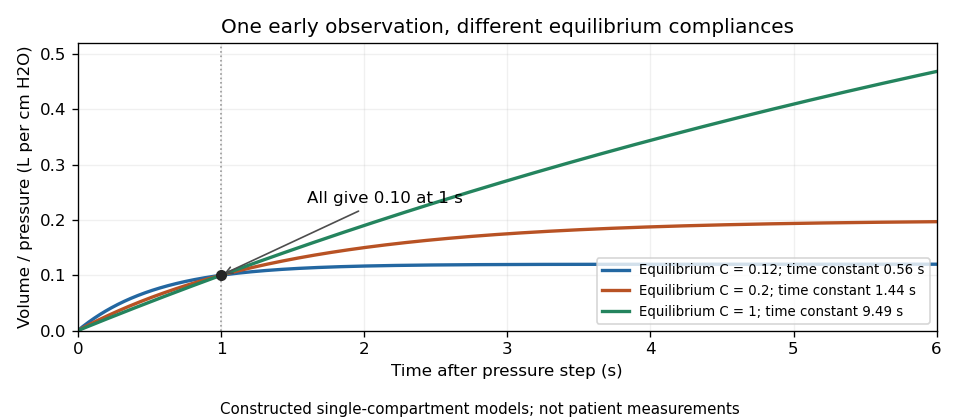
Original passive models sharing one early response while predicting different equilibrium lung compliances and time constants
. Details. The effective mass in a normal-contact penalty mode is the inertia seen by one specified relative normal displacement, rather than automatically the total mass of either body. A contact away from a center of mass can excite rotation as well as translation, changing that inertia and the normal contact penalty time scale.
Use independent generalized velocities , a positive-definite mass matrix , and a normal gap whose local velocity is . A scalar normal force produces generalized force . The primary multibody formulation gives this contact-Jacobian velocity/force pairing explicitly.[ref]
Underactuated Robotics by Russ Tedrake. Multi-Body Dynamics, Contact modeling: contact Jacobian and equation with generalized force J-transpose times lambda
At a frozen configuration, the part of gap acceleration caused by that force isIf the scalar is positive, defineThe definition uses a physical normal gap measured in metres and a matching normal force measured in newtons. Arbitrarily rescaling the gap coordinate changes the associated inertia. Constraints must first be accounted for by independent coordinates or the appropriate constrained response.A short normal impulse gives , hence . This supplies a direct interpretation: less effective mass means a larger relative normal-velocity change for the same impulse. At a fixed local configuration, a compressed linear penalty spring of stiffness gives the small-motion estimateIt omits changing contact geometry, other driving forces and damping; the source separately explains why stiff compliant contact challenges numerical integration.[ref]
For two freely translating particles, the relative gap sees , so . This is the reduced mass. Equal particles give ; replacing one by a fixed wall gives instead.
For a planar rigid body above a fixed plane, let its mass be , rotational moment of inertia about its center be , and the contact normal be vertical. A contact a horizontal distance from the center hasFor , and , . At the center it is . With , the off-center angular frequency is , compared with at the center. Using the full mass in both cases misses this rotational response.
Several simultaneous contacts require more than separate scalar replacements. Their matrix generally has off-diagonal terms: a force at one contact changes another contact’s acceleration. With frozen geometry and positive diagonal stiffness matrix , compressed gap perturbations satisfy ; its nonzero modal squared frequencies are those of the symmetric matrix . Coupled normal-contact penalty modes can therefore be faster than estimates treating each contact independently. A proposed verification applies a small known impulse or displacement perturbation at a stated configuration and checks relative contact motion, followed by a timestep convergence study.
For two configurations , the weighted Hamming distance for the noisy voter model is , where is the stationary distribution of the copying walk. On a connected undirected graph, . Positive weights make this a metric, with values between zero and one.
Couple two chains using the same uniformly selected vertex, refresh decision, fresh bit and copied neighbor. If the refresh probability is , stationarity gives . Copying redistributes disagreements without increasing their stationary-weighted total in expectation; refreshes remove them. The factor belongs to the single-vertex update convention, not a simultaneous update of every vertex.[ref]
Correlation of neighboring periodogram powers describes dependence between squared spectral magnitudes estimated from the same random record. Their dependence is not determined by the sign of amplitude covariance. A negative correlation between complex Fourier amplitudes can produce a positive correlation between their powers, changing the precision obtained by averaging nearby spectral values.
Let be zero-mean jointly Gaussian complex Fourier estimates. Define their complex covariance and nonconjugated second moment byand put . Applying Isserlis's theorem to the four factors gives three pairings:Subtracting the product of the means therefore yieldsIn particular, Gaussian power covariance is nonnegative even when a complex amplitude covariance is negative. Also ; ignoring the pseudo-covariance of a complex random variable changes the answer when that term is present.
Consider independent sample noise with independent Gaussian real and imaginary components of equal variance. Its nonconjugated moments vanish, so after any deterministic complex linear transform. If the normalized bin variances are all , thenFor the periodic Hann window with on the original -point Fourier grid, noise covariance between windowed Fourier bins gives amplitude covariance ratios at separation one and at separation two. The corresponding power correlations are and . More distant nonconjugate bins have zero covariance in that particular model.
An original calculation averages consecutive powers without wrapping around the Fourier grid. Assume so that the block does not acquire additional cyclic neighbor pairs. Counting the adjacent pairs and second-neighbor pairs givesFor , the variance is , rather than the independent-value result . For , it is , rather than . A variance-equivalent independent-power count is the reciprocal of this normalized variance: about for those ten bins. For , the bracket simplifies to , approaching roughly independent powers for large blocks in sufficiently long records.
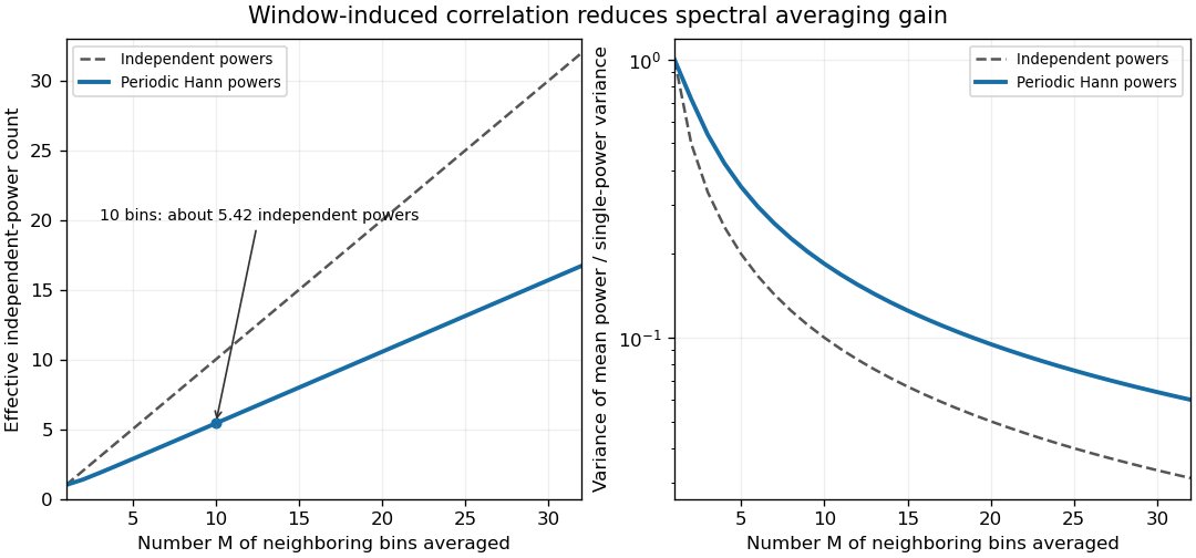
Correlated periodic Hann window powers give less variance reduction than independent spectral powers
. Exact finite-block variance and variance-equivalent independent-power count for Gaussian complex white sample noise on the original N=64 grid. Blocks contain one to 32 consecutive bins, so the plotted calculation has no extra wraparound pairs. Each variance is normalized by its model’s single-power variance. The lines are analytical predictions, not experimental observations. Details.Real-valued Gaussian input has conjugate Fourier symmetry and can have nonzero , especially for mirrored frequencies and endpoint bins. A deterministic spectral component also invalidates the zero-mean calculation unless its additional mean-dependent terms are included. Colored noise, taper convention and detrending change and ; the formulas above do not make all measured spectra follow one correlation pattern.
A periodogram may be expressed as a squared spectrum or a power spectral density. SciPy documents their window-dependent conversion, one-sided folding and optional detrending explicitly.[ref]
SciPy 1.16.2 documentation. scipy.signal.periodogram, scaling, return_onesided and detrend parameters; Notes
A common positive scaling does not change the correlation coefficient, but combining unequal scalings or folding conjugate values requires carrying those transformations through the covariance.A proposed check generates independent records under the stated noise model, calculates bin powers with the same window, and compares empirical pair covariances and block-average variance with the predictions. Independent records provide a different averaging resource from additional bins or zero-padded frequency points in one record. Report which values were averaged and their covariance before assigning an independent-sample precision gain.
Long short-term memory, usually abbreviated LSTM, is a recurrent neural network architecture that carries an explicit memory state through a sequence and learns when to write, retain and expose its contents. It addresses the vanishing gradient problem: in ordinary recurrence, repeated multiplication by small derivatives can make a distant input have almost no effect on the gradient used for learning. Sepp Hochreiter and Jürgen Schmidhuber's 1997 architecture provided a memory-cell path designed to preserve error flow, with gates controlling access.[ref]
Long Short-Term Memory by Sepp Hochreiter and Jürgen Schmidhuber. Abstract and memory-cell construction: constant error flow and input/output gates.
A common simplified modern form, omitting peephole connections, isHere is the input, the memory, the exposed state, the logistic sigmoid function, the hyperbolic tangent, and componentwise multiplication. The learned matrices and biases determine an input gate in long short-term memory , a forget gate in long short-term memory , and an output gate in long short-term memory . LSTM: A Search Space Odyssey by Klaus Greff and others gives a more general baseline with peephole connections; the equations above deliberately show the simpler variant.[ref]
LSTM: A Search Space Odyssey by Klaus Greff and others. Section II and Figure 1: gate roles and baseline update equations.
For a scalar memory with writing switched off in the idealized limit and constant retention , . Over 100 steps, retains about , while retains about . This illustrates how a learned gate can select a retention timescale. Exactly zero or one are limiting idealizations for a finite-input logistic sigmoid function. The product of forget gates describes the direct memory path; it is not the entire recurrent derivative, because gates also depend on earlier states.
The forget gate in long short-term memory was introduced after the original architecture, in Learning to Forget: Continual Prediction with LSTM by Felix A. Gers, Jürgen Schmidhuber and Fred Cummins, to allow old contents to be reset during continuing input streams. Training still uses methods such as backpropagation through time. Artificial delayed-dependency tasks in the original paper demonstrated learning across more than 1,000 time steps in particular experiments; this does not imply unlimited memory or guaranteed success on every long sequence.[ref]
Learning to Forget: Continual Prediction with LSTM by Felix A. Gers, Jürgen Schmidhuber and Fred Cummins. Abstract and adaptive forget-gate motivation.
[ref]Long Short-Term Memory by Sepp Hochreiter and Jürgen Schmidhuber. Abstract and long-delay task experiments.
A neural network logit is a real-valued class score produced before a probability transformation such as the softmax function. The vector of scores determines the class probabilities jointly; an isolated score is not itself a probability. Negative scores and scores larger than one are permitted.[ref]
On Calibration of Modern Neural Networks by Chuan Guo and others. §4.2, paragraph before Eq. (8), logits before the softmax layer
For scores , the softmax function givesAdding one common scalar to every coordinate leaves all probabilities unchanged:Consequently the absolute offset of a logit vector cannot be recovered from these probabilities.
For example, scores and both give first-class probability . The difference between the two scores, rather than the first coordinate alone, determines this binary probability. Indeed,This connects the binary score difference with the logit link function. It does not make every coordinate of a multiclass score vector a separately defined binary log-odds.
A common shift also differs from rescaling. Dividing by two gives and first-class probability . This is the transformation used in temperature scaling with temperature two. Positive scaling preserves the selected class within an example while changing confidence.[ref]
When interpreting a neural network logit, state its score vector and probability transformation. Comparing raw coordinates from independently shifted parameterizations can otherwise suggest a confidence change where the actual probability vector is identical.
A Mycielski graph commonly means a member of the family obtained by repeatedly applying the Mycielski construction to . Writing and , its chromatic number is , although it has no triangle. More broadly, the term is sometimes used for a graph produced by that construction from another starting graph; the chosen family convention should be stated.
The first examples are , , and the eleven-vertex . Each construction adds a shadow for every old vertex and one apex, so the vertex counts satisfy . Hence .
These graphs demonstrate that forbidding triangles in a graph does not bound the number of colors needed. A large clique is only one obstruction to coloring: constraints spread through a triangle-free graph can force arbitrarily large chromatic number.
The polynomial model of a regularity structure realizes abstract monomials as ordinary coordinate differences around each base point. It is the example that turns a regularity structure into familiar Taylor polynomials. In dimensions, use a polynomial ring in symbols , graded by total degree. For a multi-index ,Re-expansion uses . Substitution immediately gives and , the compatibility identities of a model of a regularity structure.[ref]
A theory of regularity structures by Martin Hairer. §2.2, polynomial regularity structure; §2.3, Definition 2.17 and Remark 2.23, canonical polynomial model
For example, has local abstract expansion at . At it has . Transporting the latter substitutes :The coefficients change because the expansion point changes; the represented function is still .
The analytic scaling also follows by calculation. For a smooth test function and , changing variables givesThus the assigned degree predicts exactly the power of in the model bound. Anisotropic scaling can assign different weights to different coordinates instead; ordinary total degree is the isotropic choice. General regularity structures retain this organization of local expansions while admitting symbols that are not polynomials.
Batch size counts the examples combined in a mini-batch. In the simple stochastic gradient descent loop where each group produces one parameter update, it controls how many examples contribute to that update. It differs from a training epoch, which counts a pass over the available training data.[ref]
Optimizing Model Parameters in the PyTorch tutorials. Hyperparameters and Optimization Loop
For an original counting example, partition ten examples with nominal batch size and retain the remainder. The actual sizes are , giving updates per training epoch. Discarding the remainder instead gives two updates and uses only eight examples. More generally the retained-remainder update count is for examples, provided there is one update per group.
Batch size also changes gradient sampling noise. If independently sampled component gradients at a fixed parameter have scalar variance , their sample mean hasFor an original exact example, suppose one component gradient is equally likely to be 0 or 2. Its mean is 1 and variance is 1. A two-example mini-batch gradient takes values with probabilities , giving variance . This calculation holds parameters fixed and assumes independent sampling; sampling without replacement has a finite population correction.
With gradient accumulation, several groups may contribute before an update. Two full four-example groups then involve eight examples per update if their gradients are normalized consistently. State whether a reported size counts the processed group or all examples contributing to an update. Lower sampling variance alone does not establish faster training for a fixed computation budget.
An air-displacement pipette uses a piston to change the pressure and volume of an air cushion above a liquid sample. On piston withdrawal, reduced pressure allows ambient pressure to drive liquid into the tip; subsequent piston motion expels it. The piston itself remains separated from the sample.[ref]
Gilson Guide to Pipetting. second edition, pp. 8–11, air-cushion mechanism and aspiration/dispensing sequence
The air cushion explains why a mechanical setting alone does not establish the delivered volume. Its response can depend on temperature and sample properties, including volatility and density. A positive-displacement pipette uses direct piston contact instead of that intervening gas volume.[ref]
Gilson Guide to Pipetting. pp. 9–12, contrast between mechanisms and influence of sample properties
For an original repeated-delivery example, compare sets of settings with measured mean deliveries of and . Knowing those means alone does not identify which set has less scatter. Both the mean error and a dispersion measure such as standard deviation are needed to describe performance. A microlitre is an exact unit relationship; an individual micropipette delivery is an experimental measurement.
A positive-displacement pipette transfers liquid with a piston that contacts the sample directly, avoiding the intermediate air cushion of an air-displacement pipette. In the handheld designs described by the manufacturer, the capillary and piston form a disposable assembly. The mechanism can reduce effects associated with the expansion or contraction of trapped air.[ref]
Gilson Guide to Pipetting. second edition, pp. 8–11, positive-displacement construction and operation
This distinction is useful when handling liquids whose viscosity, density or volatility differs substantially from water. The instrument still measures a volume: a selected does not imply a fixed mass for every liquid. For an illustrative density of , the corresponding mass is by .
A gravimetric check therefore needs the appropriate density conversion. Direct displacement also does not make every delivery perfect: instrument condition, the fitted assembly and the test procedure remain relevant. Repeated measurements distinguish a systematic displacement of the mean from scatter in individual deliveries.[ref]
Gilson Guide to Pipetting. pp. 46–49, performance assessment and gravimetric procedure
A microbial cryoprotectant is a substance added to help viable microorganisms withstand freezing and subsequent recovery during microbial cryopreservation. Protection is assessed in the preserved material; the label does not mean that a substance is harmless at every concentration or suitable for every strain.
Freezing changes both the amount of liquid water and the concentration of dissolved substances. Intracellular ice can injure structures, while water movement by osmosis can shrink a cell. ATCC identifies glycerol and dimethyl sulfoxide as common protective agents and stresses that useful formulations depend on the material. Protecting a frozen preparation involves more than simply lowering its nominal temperature.[ref]
Mycology Culture Guide by ATCC. Preservation: Cryopreservation, Overview and Freeze Medium
An original comparison measures recovery rather than assuming protection from composition. Split a benign yeast preparation into two matched portions. Suppose each has1000 initial colony-forming units per original-volume equivalent, while recovery gives300 units without a candidate additive and700 with it. The recovered fractions are0.30 and0.70: a difference of0.40, or40 percentage points, and a ratio . These invented measurements would support improved recovery in that comparison, not a universal survival rate.
Equal original-volume equivalents matter because adding a solution also dilutes the cells. A matched nonfrozen comparison can help separate freezing injury from an additive's effect on the growth readout. Recovery of colony-forming units, unchanged genotype and preservation of a chosen phenotype are separate questions.
The practical motivation is to retain a reproducible biological starting point between experiments. A microbial cryoprotectant is one part of that preservation system, alongside the physical freezing history, storage and subsequent authentication.[ref]
Bacteriology Culture Guide by ATCC. Preservation and Bacterial Authentication
The Metropolis algorithm is the symmetric-proposal case of the Metropolis–Hastings algorithm. At state with positive target density , propose from with , and accept with probabilityOtherwise remain at . A normalizing constant in cancels, which makes the method useful when a target distribution is known only up to scale.
The accepted probability flow is , symmetric in . This proves detailed balance and hence invariance of the target under the usual kernel assumptions.
For two states with target masses and an always-flip proposal, moves from the first state are always accepted, while reverse moves are accepted with probability . The rejection probability creates holding at the second state. Target invariance alone does not prove convergence from every start; irreducibility and appropriate periodicity conditions matter. An asymmetric proposal requires the Hastings proposal-density correction.
Pinned article: Introduction to the OurBigBook Project
Welcome to the OurBigBook Project! Our goal is to create the perfect publishing platform for STEM subjects, and get university-level students to write the best free STEM tutorials ever.
Everyone is welcome to create an account and play with the site: ourbigbook.com/go/register. We belive that students themselves can write amazing tutorials, but teachers are welcome too. You can write about anything you want, it doesn't have to be STEM or even educational. Silly test content is very welcome and you won't be penalized in any way. Just keep it legal!
Intro to OurBigBook
. Source. We have two killer features:
- topics: topics group articles by different users with the same title, e.g. here is the topic for the "Fundamental Theorem of Calculus" ourbigbook.com/go/topic/fundamental-theorem-of-calculusArticles of different users are sorted by upvote within each article page. This feature is a bit like:
- a Wikipedia where each user can have their own version of each article
- a Q&A website like Stack Overflow, where multiple people can give their views on a given topic, and the best ones are sorted by upvote. Except you don't need to wait for someone to ask first, and any topic goes, no matter how narrow or broad
This feature makes it possible for readers to find better explanations of any topic created by other writers. And it allows writers to create an explanation in a place that readers might actually find it.
Figure 1. Screenshot of the "Derivative" topic page. View it live at: ourbigbook.com/go/topic/derivativeVideo 2. OurBigBook Web topics demo. Source. - local editing: you can store all your personal knowledge base content locally in a plaintext markup format that can be edited locally and published either:This way you can be sure that even if OurBigBook.com were to go down one day (which we have no plans to do as it is quite cheap to host!), your content will still be perfectly readable as a static site.
- to OurBigBook.com to get awesome multi-user features like topics and likes
- as HTML files to a static website, which you can host yourself for free on many external providers like GitHub Pages, and remain in full control

Figure 2. You can publish local OurBigBook lightweight markup files to either OurBigBook.com or as a static website.
Figure 3. Visual Studio Code extension installation.
Figure 5. . You can also edit articles on the Web editor without installing anything locally. Video 3. Edit locally and publish demo. Source. This shows editing OurBigBook Markup and publishing it using the Visual Studio Code extension. 
- Infinitely deep tables of contents:




All our software is open source and hosted at: github.com/ourbigbook/ourbigbook
Further documentation can be found at: docs.ourbigbook.com
Feel free to reach our to us for any help or suggestions: docs.ourbigbook.com/#contact