Topics (384k) Articles (398k) Users (410) Discussions (242) Comments (383) Files (13k) New article

A defier is a unit with potential treatment receipts and : it takes the treatment without encouragement but does not take it when encouraged. This is the principal stratum. The word specifies potential behavior under a particular binary intervention; it does not describe a general personality trait.
A defier contributes to , whereas a complier contributes . Consequently,The usual instrumental-variable monotonicity assumption sets the second probability to zero. A positive average effect of encouragement on receipt does not prove that there are no defiers: positive and negative individual changes can coexist.[ref]
A complier is a unit with potential treatment receipts and : binary encouragement changes its receipt from no treatment to treatment. This pair defines a principal stratum, rather than a behavior inferred from one observed assignment.
For example, a unit that participates exactly when invited is a complier. Under instrumental-variable monotonicity, which excludes defiers,Thus, with randomized assignment, the difference in treatment-receipt rates estimates the complier fraction. To interpret an outcome-rate ratio as the local average treatment effect, one additionally needs the relevant independence and exclusion assumptions and a nonzero complier fraction. An observed encouraged participant may instead be an always-taker.[ref]
Principal Stratification in Causal Inference by Constantine E. Frangakis and Donald B. Rubin. Section 2, cross-classification by intermediate potential values
A never-taker is a unit whose potential treatment receipts are : it receives no treatment under either value of a binary assignment or encouragement . This is the principal stratum, defined before observing which assignment actually occurs.
For example, a unit may decline participation whether or not it receives an invitation. Among units with observed , never-takers are mixed with compliers, so a single observation does not reveal the principal stratum. Under an exclusion restriction through treatment receipt, assignment has no outcome effect on a never-taker because receipt stays fixed; that is an additional causal assumption, not part of the definition.[ref]
Principal Stratification in Causal Inference by Constantine E. Frangakis and Donald B. Rubin. Section 2, principal strata defined by joint intermediate potential values
An affine pressure-tap coordinate calibration converts an instrument coordinate to a physical coordinate through an affine map, . The offset fixes the datum and the nonzero scale fixes the length conversion. Its adequacy is a question about the actual viewing or measuring geometry, rather than a consequence of having fitted two points.
For two distinct instrument readings at known physical references ,An original imaging example takes the leading edge at pixels and , and the trailing edge at pixels and m. Hence m/pixel and m. A tap at pixels is at m, or dimensionless chord position .
If all three features share the same affine map, the dimensionless coordinate is simplyChanging the displayed coordinate to gives readings 230, 1030 and 470 pixels and leaves . This is the exact pressure-tap datum cancellation; it does not assert that the original feature readings are known without uncertainty.
For example, with , the sensitivity coefficients of with respect to the tap, leading-edge and trailing-edge readings areTheir sum is zero, as required for invariance to a common offset. At the example readings they are per pixel. Use their full covariance matrix when propagating uncertainty, because independently attaching three origin errors would destroy the cancellation.[ref]
Guidelines for Evaluating and Expressing the Uncertainty of NIST Measurement Results by Barry N. Taylor and Chris E. Kuyatt. Appendix A, covariance terms in the measurement-model sensitivity law
An affine pressure-tap fiducial check uses an additional independently located mark. At pixels the fitted map predicts m. A measured location m leaves a 2 mm discrepancy to investigate. Two fitted reference points necessarily have zero regression residual; that fact cannot validate the map between them. Perspective, surface curvature, optical distortion and reference-location uncertainty can all matter. A proposed calibration records extra marks across the image and compares residual patterns before using the map for surface pressure integration for airfoil lift.
Uniform coverage over confidence-allocation choices means that one probability statement protects every allocation in a specified family simultaneously. For upper bounds on a parameter , the required statement isIt implies coverage for the minimum selected after observing the data. Separate statements for each fixed do not imply the simultaneous statement. The difference is the order of the probability and the requirement to cover every choice.
For a finite set of candidates, assigning each a failure budget and applying the union bound provides uniform protection. This is the simultaneous-coverage principle behind the Bonferroni correction.[ref] A continuum requires a family-level argument rather than multiplying one finite-candidate budget by an undefined number of choices.
An original construction exploits nested one-sided bounds in the detection model . Suppose decreases as its failure budget increases, and increases as increases. Choose allocations , , with . On the common eventevery candidate ratio bounds . The union bound controls this common event's failure probability byThis extremal calibration for nested confidence families protects the entire interval of allocations using just its most demanding marginal endpoints.
For example, take , and . Each fixed allocation has at least 96% coverage, while the common-event argument guarantees at least 95% coverage for every allocation simultaneously. Selecting the smallest bound within that prespecified interval is therefore protected at the latter level, without assuming independence of the marginal bounds.
The proof depends on the nesting, valid marginal bounds and a specified family. Enlarging the family after inspecting the observations needs corresponding protection. Where a lower detection bound can be zero, the prevalence upper bound must revert to the uninformative value one rather than divide by zero.
Carbon-basis closure for polymer degradation compares the amount of carbon initially introduced in a polymer with the carbon recovered in all measured products and residues. It avoids confusing incorporated water with recovered original polymer mass, while requiring dissolved and gaseous products to be counted as well as retained solids.
On a consistent specimen-carbon basis, writeThe measured recovery is the sum of the first four terms divided by . Specify whether each denotes carbon mass or amount of substance; numerator and denominator must use the same units. Carbon from medium, inoculum, solvent or contamination must be separated from specimen-derived carbon.
An original polyglycolic acid example begins with one millimole of repeat-unit inventory, containing two millimoles of carbon atoms, approximately 24.02 mg of carbon. Hydrolysis to one millimole of glycolic acid preserves those carbon atoms while incorporating water. The product's larger total mass is therefore not extra carbon recovery. The manufacturer's repeat structure and decomposition diagram identify that chemical relationship.[ref]
Kuredux Polyglycolic Acid Resin technical brochure by Kureha. PDF p. 2, Molecular Structure and decomposition diagram
If some products become carbon dioxide, convert measured gas mass to carbon mass before adding it to residue carbon:For an illustrative initial 24 mg of carbon, suppose corrected measurements recover 12 mg in solid, 6 mg dissolved and approximately 3 mg in carbon dioxide. Recovery is , leaving 3 mg unaccounted. Approximately 11 mg of carbon dioxide contains 3 mg of carbon; adding that full gas mass to solid and dissolved carbon would mix bases.
A concrete primary apparatus is the OECD 301 B carbon-dioxide evolution test. It aerates inoculated mineral medium with carbon-dioxide-free air at a controlled rate, traps evolved gas in barium or sodium hydroxide, and determines it by titration or inorganic-carbon measurement. Blank inoculum contributions are subtracted.[ref] These operations explain why inlet scrubbing, gas collection and blank correction belong to the measurement rather than being optional bookkeeping.
The guideline is a chemical biodegradability test, not proof that every polymer shape or formulation meets its applicability conditions. Its general section requires attention to solubility, volatility, adsorption and composition.[ref]
Test No. 301: Ready Biodegradability by OECD. General procedures, §§7–9
Use those conditions when adapting a collection experiment to a particular specimen.Blank-corrected carbon recovery in polymer tests also needs uncertainty in the background subtraction. Carbon missing from the liquid can have moved to surfaces or gas without being completely converted to carbon dioxide. Conversely, carbon dioxide production establishes conversion of some carbon but does not measure the remaining chain-length distribution. Report closure, identified chemical products and the molar mass distribution as different results; a successful elemental balance alone does not determine the degradation mechanism.
Asynchronous pin release ends the address-stability guarantee for a pinned memory object after an operation that can continue beyond its submission call. Its central condition is that no unfinished consumer may still access the pinned address. Returning from submission is sufficient only when the operation's contract says that all access has ended. Microsoft's asynchronous native-call example stores the pin handle in callback state and disposes it during completion cleanup.[ref]
Memory and Span usage guidelines by Microsoft. Rule10, asynchronous native-call wrapper and completion callback
For an original event sequence, suppose an operation acquires a pin at0ms, submits at1ms, returns a pending result at2ms and finishes its last access at8ms. Completion cleanup at8ms can end the pinning lifetime; cleanup at2ms cannot. If a request to stop arrives at3ms but the operation acknowledges completion only at6ms, the request alone does not authorize release at3ms. The actual access contract, rather than the desired outcome, determines when the address may change.
An implementation needs a single owner for cleanup across all completion paths. Submission might fail before any callback is promised, complete immediately, or complete later. Each path must transfer or retain the cleanup responsibility consistently. The exactly-once pin cleanup requirement avoids both leaking a pin and releasing the same handle twice. The primary Microsoft example explicitly cleans up an exception before a callback can be invoked, and funnels immediate and deferred completion through a completion routine.[ref]
Memory and Span usage guidelines by Microsoft. Rule10, exception cleanup and non-pending completion branch
With overlapping users, releasing one operation's interest does not establish that every user has finished. A reference counting protocol can track outstanding access leases, provided starting new work and deciding that the last lease ended are synchronized. An observed zero count without protection against a simultaneous new user is not sufficient. A mutex or another appropriate synchronization mechanism can protect that transition.
The completion signal must itself describe the end of access. Microsoft's task-based buffer rule forbids a consumer from continuing to use the memory after the returned task reaches a terminal state.[ref]
Memory and Span usage guidelines by Microsoft. Rule4, consumer lifetime and task terminal state
An API that reports cancellation before its underlying user has stopped requires another completion guarantee before pin cleanup. Retaining the pin protects the address; it does not by itself prevent concurrent data races or determine who may reuse the buffer.A piezoelectric material couples mechanical deformation with electric polarization. In a linear small-signal description, one convention writes : applied stress contributes to electric displacement. The converse effect produces strain when an electric field is applied.
A quartz element can generate an electrical signal under mechanical loading, while an applied alternating voltage can drive a mechanical resonance. This reciprocity makes piezoelectric materials useful for sensors, actuators and frequency control. The coefficients depend on direction and crystal symmetry; an isotropic scalar coefficient cannot describe every orientation of a single crystal.
Photoresistor spectral calibration determines how a photoresistor's electrical reading depends on the illumination spectrum under specified geometry, background, temperature, bias and adaptation history. A resistance-versus-lux curve measured with one lamp is not automatically valid for another spectrum. The manufacturer's primary CdS datasheet specifies a source for its light-resistance tests and preconditions cells with light before electrical measurements.[ref]
NSL-5162 CdS photoresistor datasheet by Advanced Photonix. page 2, light-resistance test conditions and adaptation footnote
The distinction is between irradiance and illuminance. With spectral irradiance , illuminance is approximatelywhere is the photopic luminous efficiency function. The detector weights wavelengths according to its own physical response, which need not be proportional to . NIST's detector-based photometric realization measures that spectral response, rather than assuming an arbitrary detector reproduces the photometric weighting.[ref]
Realization of the candela. Detector-based realization, illuminance responsivity and spectral integrals
For a locally linear small-signal model about a fixed operating state, writeHere is the differential spectral responsivity of electrical conductance, including the stated illumination geometry. It is not automatically a global, illumination-independent material constant. A background-dependent photoresistor spectral response requires rechecking this derivative when the operating point changes.
An original two-band example makes the mismatch quantitative. Stipulate relative photometric weights , and equal detector generation weights for two narrow bands. Equal illuminance requires four times as much irradiance in band , so its detector-weighted generation is four times greater. If, over this illustrative range, , the resistance ratio is . These weights and exponent are stipulated, not measured specifications or tabulated values for named wavelengths. Equal lux can produce substantially unequal resistance.
A proposed spectral characterization uses narrow-band sources or a monochromator, a reference detector to measure incident irradiance, fixed beam geometry and controlled detector temperature. Record resistance or conductance after a defined settling time at several background levels. A separate calibrated photometer can establish illuminance; it cannot by itself establish the photoresistor's spectral weighting. Keep electrical loading and self-heating fixed while changing the source.
For a broadband transfer, characterize the reference and test spectra and test whether the measured spectral-response model predicts their relative readings. Existing spectral mismatch correction methods address the analogous transfer problem for photometers, but a nonlinear photoresistor first needs a justified operating-point model.[ref]
NIST Measurement Services: Photometric Calibrations by Yuqin Zong and others. §3.4.3, equation 22, and §3.6.2, spectral mismatch for sources different from the calibration lamp
The result is a calibration valid for stated conditions, not a universal conversion from resistance to optical power.Photoconductor rise and fall asymmetry means that a photoconductor's normalized turn-on and turn-off transients have different shapes or threshold-crossing durations under stated illumination and electrical conditions. Define the levels first: a ten-to-ninety-percent rise and a ninety-to-ten-percent fall exclude different portions of a long tail than a zero-to-ninety-percent measurement. Detector temperature is an essential condition because the primary PbS description reports changes in response speed, dark resistance and spectral sensitivity with temperature.[ref]
How does a PbS photoconductive detector work? by Shimadzu Scientific Instruments. temperature-dependence paragraph
The simplest linear carrier model predicts symmetry. For excess carrier density satisfying , a step to gives ; switching off after equilibration gives . Both threshold durations equal . Thus different measured durations are evidence against that complete one-pole measurement model, rather than a result it already predicts.
A photoconductor transient with quadratic recombination supplies an illuminating alternative model. Stipulate constant mobility, fixed detector bias, zero dark excess density andUnder constant , let and . Starting at zero gives . Starting at and setting gives . Direct substitution verifies both solutions.
For an output proportional to , the resulting durations areWith stipulated , the rise takes and the fall , despite having no separate fitted rise and fall constants. This is a derived nonlinear electron-hole recombination model, not measured behavior or a specification of the cited PbS or CdS detector. Its long algebraic tail also shows why a single exponential fit may depend strongly on the fitted interval.
The readout can itself introduce asymmetry. A resistance divider has output as a function of detector electrical conductance . Equal exponential rise and fall in need not give equal normalized threshold durations after this nonlinear conversion. Carrier dynamics, the electrical transfer curve and an amplifier's response must therefore be separated before assigning a material lifetime.
A proposed experiment switches a monitored optical source between two reproducible levels, measures actual detector bias and current, waits for the same initial equilibrium, and repeats in both directions. Compare current-derived conductance with divider output, then vary background, temperature and step size. A slow reference source or readout can imitate a detector tail. Asymmetry alone does not uniquely identify trapping or any other microscopic mechanism.
Four-step phase retrieval estimates relative wave phase from four wave interference frames separated by quarter-cycle wave phase steps. Use the explicit signal-arm conventionwith a common background and modulation amplitude . Opposite-frame differences giveso . The order of the subtractions fixes the sign. Changing which arm receives the wave phase step requires a correspondingly changed convention.
The same data estimate and . A simple model-consistency residual is , which is zero for the exact stated model. It does not detect every possible systematic error.
For an original example, let , and . The four light intensities are , , and . Then , , and the recovered wave phase is . Common background cancels, whereas changing background separately between frames need not cancel.
If independent additive errors in the four light intensities have common variance , first-order propagation givesThis follows from and difference variances . It applies away from vanishing modulation and assumes the specified independent equal-noise model. wave phase uncertainty grows when interference visibility is weak.
The method is a discrete instance of phase-shifting interferometry, whose early digital apparatus used controlled reference-path modulation and synchronous wave phase extraction.[ref]
Digital Wavefront Measuring Interferometer for Testing Optical Surfaces and Lenses by J. H. Bruning and others. Abstract, reference-arm modulation and Fourier-series detection; the four-frame derivation here is separate
The result is still a principal wave phase; phase unwrapping cannot be replaced by choosing a different arctangent branch at each pixel without a consistency rule.At fixed temperature and pressure, liquid-liquid equilibrium is stable coexistence of distinct liquid thermodynamic phases that minimizes total Gibbs free energy for the specified component amounts. Their compositions can differ even though each exchanging chemical species has the same chemical potential in both phases. For neutral, nonreacting components in bulk phases at common temperature and pressure , neglecting external-field and interface-curvature contributions,To see why, transfer an amount from phase to phase while holding the total amount of each component fixed. The change in Gibbs free energy is . If the coefficient is nonzero, one transfer direction lowers . Equality removes that driving term; stable equilibrium additionally requires a global minimum over the allowed phase arrangements. Here each chemical potential is the partial derivative of Gibbs free energy with respect to that component amount at fixed temperature, pressure and the other component amounts.[ref]
Charged species instead require equality of the corresponding electrochemical potential. Equal chemical potentials for neutral species do not require equal mole fractions. With a common pure-component reference, and , where is thermodynamic activity, an activity coefficient, and the molar gas constant. The activity equality for coexisting liquids is . Different nonideal environments can therefore support different compositions at the same chemical potential.
For a binary mixture, let be the mole fraction of component B and let be the homogeneous molar Gibbs free energy at fixed . Differentiating givesEquality of both component chemical potentials between two compositions becomes the common-tangent construction for phase coexistence:In this molar representation, the tangent slope is and its intercept is . Stable coexistence uses a supporting tangent lying below the homogeneous curve over all admissible compositions. This constructs the relevant convex envelope; two stationary points or equal slopes alone do not establish stability.
An original regular solution calculation makes this distinction visible. Because linear composition bias leaves coexistence compositions unchanged, subtract the linear pure-component reference and writeThe dimensionless parameter penalizes unlike contacts when it is positive. Take . Symmetry makes the coexistence tangent horizontal, and the two outer solutions of give the symmetric regular-solution binodal:These are model compositions, rather than measured hexane–water values. At overall mole fraction , the liquid-liquid tie line and lever rule give the fraction of total moles in phase :Changing within the coexistence interval changes phase amounts while leaving the two endpoint compositions fixed. These mole-based phase fractions need not equal volume fractions.
The spinodal answers a different question: local stability of a homogeneous mixture. Here , so at the two local-stability limits are . Between them, composition fluctuations lower the bulk free energy. Between a binodal endpoint and the nearer spinodal, the homogeneous state has positive local curvature but a lower-energy phase-separated state exists: this is metastability. Thus the observed coexistence compositions are not obtained merely by setting .
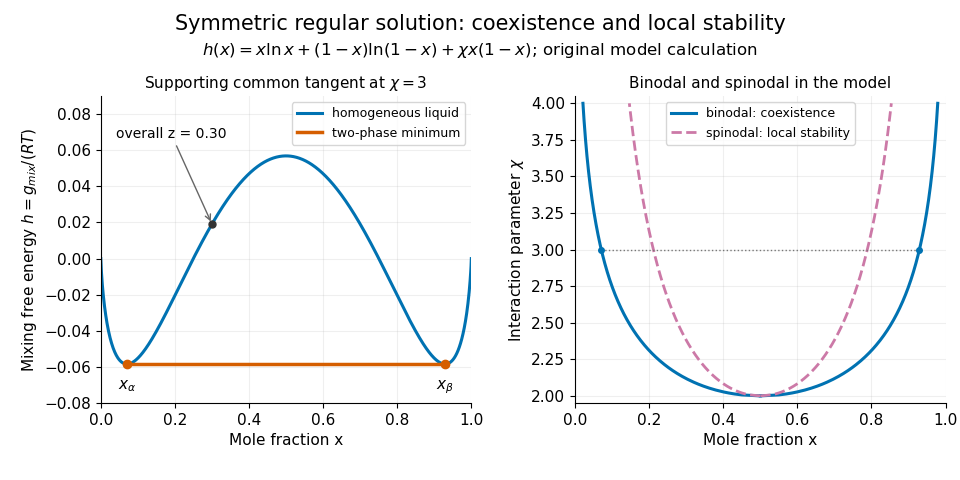
Original regular-solution model: the supporting tangent gives liquid coexistence, while the spinodal marks loss of local homogeneous stability.
Details. A useful experiment measures compositions as well as the presence of layers. One hexane–water record reports overnight shaking, microsyringe sampling of the aqueous solution, and gas chromatography to measure dissolved hydrocarbon. The small dissolved amount is evidence of finite mutual solubility, consistent with liquid immiscibility over other bulk compositions.[ref]
Hexane with water in the IUPAC-NIST Solubility Database. Record37_269, Experimental Data and Method/Apparatus/Procedure; no ambiguous table values are used here
At controlled temperature, repeated sampling of both phases and checks from different initial compositions help test whether the endpoint compositions have stabilized. Critically evaluated reference systems provide a way to validate such instruments and techniques.[ref]Reference Materials for Phase Equilibrium Studies. 1. Liquid-Liquid Equilibria by Ala Bazyleva and others. Abstract and Introduction: seven binary reference systems, accepted data and uncertainty estimates
A phagolysosome is a degradative, particle-containing compartment formed as a phagosome matures through interactions with endosomes and lysosomes. After phagocytosis, the engulfed particle can remain recognizable while its surrounding membrane and contents change. The particle's identity therefore does not establish the biochemical state of the whole compartment.[ref]
Biogenesis of phagolysosomes proceeds through a sequential series of interactions with the endocytic apparatus by M. Desjardins and others. Abstract and Figures 5–7, sequential changes in latex-bead-containing compartments
A useful experiment followed low-density latex beads taken up by J774 macrophages. The bead-containing compartments were isolated by flotation on a sucrose gradient. In a pulse-chase analysis, a limited uptake period followed by different waiting intervals yielded compartments of different ages. Comparing their proteins and immunogold labeling revealed changing membrane composition during maturation.[ref]
Biogenesis of phagolysosomes proceeds through a sequential series of interactions with the endocytic apparatus by M. Desjardins and others. Figure 6 and Table I, LAMP2 immunogold labeling after the bead pulse and chase; Figures 5–7
Normalization matters when interpreting such images. With invented counts, 10 gold labels along of membrane give labels per micrometre; 20 labels along give only label per micrometre. The second sample has more total labels but a smaller label density. Comparing membrane lengths prevents the amount of membrane observed from being mistaken for the abundance of its marker.
That measurement concerns localization of a membrane marker. It is not itself a measurement of luminal pH, degradation rate or killing of a microorganism. Those functions need corresponding observations: acquisition of one marker and completion of a degradative process answer different experimental questions.
The percolation susceptibility exponent describes how the expected finite-cluster size diverges on approaching the percolation critical probability from below. If is the percolation susceptibility and a power law holds, thenEquivalently, . A stronger statement also specifies an amplitude ; existence of either form needs justification for the model in question.
For bond percolation on an infinite -regular tree, , there are vertices at distance from the root and a unique path to each. For ,Thus and . This solvable geometry explains the simplest divergence, while more complicated lattices need not share its exponent. The tree-graph moment bound for a percolation cluster gives a route to proving the value one under suitable diagrammatic conditions.[ref]
Tree graph inequalities and critical behavior in percolation models by Michael Aizenman and Charles M. Newman. Abstract and susceptibility criterion
Optical energy outside a time gate is the radiant energy excluded by a specified ideal temporal acceptance set . For a nonnegative radiant power profile of finite positive total energy,The time-integral definition is the radiometric one.[ref]
International Lighting Vocabulary by CIE. entry17-21-041, note1, radiant energy as the integral of radiant flux
This observable needs a gate boundary but no fitted separation into a main field and an optical pulse pedestal.For an original three-pulse example, let an optical prepulse, main pulse and optical postpulse carry , and respectively, with disjoint supports. A gate containing only the main pulse admits of , so . Widening that gate to include the postpulse reduces the fraction to . The optical waveform has not changed; the admitted observable has.
For a translated interval with continuous boundary values,Unequal power at the boundaries produces first-order sensitivity to a timing shift. Equal boundary values eliminate this derivative but need not eliminate higher-order loss; quadratic energy loss from centred Gaussian gate timing error gives an existing example.
The total-energy denominator must cover the excluded light too. If the acquisition window misses an unknown tail, pulse-energy interval from incomplete tail measurements supplies conditional bounds rather than an exactly known fraction. A detection time gate on an electrical detector trace also includes the detector impulse response and is not automatically an ideal gate on incoming optical power. A characterized optical response and a stated detector baseline subtraction are needed to compare the two.
A mixed peak and RMS gain-calibration error occurs when input and output amplitude reports use different reconstruction scales but their numerical ratio is treated as the physical gain. Let the true peak amplitude phasors obey . If a reported amplitude reconstructs the signal with scale , so that , thenThe scale is for a peak phasor and for an RMS phasor. Equal physical units do not establish equal amplitude conventions. The sinusoidal RMS-to-peak conversion follows from the period average of the squared signal.[ref]
For a peak-normalized input and RMS-normalized output, the raw ratio is ; for the reverse pairing it is . The amplitude-gain error in decibels is therefore minus or plusThese positive real normalization factors do not themselves change the relative phase. They change the measured gain magnitude.
For an original calibration example, let a sinusoidal input be reported as peak and its output as RMS. The raw amplitude ratio is , or about . Converting the output to peak amplitude gives actual gain , or about . A source-to-receiver comparison that ignores the conventions would falsely report a gain deficit.
A further factor-of-two issue occurs when one report is a positive-frequency Fourier coefficient rather than a peak phasor; peak phasor versus positive-frequency Fourier coefficient derives that distinction. It produces a different amplitude factor and must not be treated as an RMS conversion. Likewise, peak-versus-RMS normalization in complex electrical power uses a product of reconstruction scales rather than the ratio used here. A calibration record should therefore state the sinusoidal amplitude convention and, for sampled estimates, the FFT normalization before numerical gains are compared.
Finite-record phasor extraction with coherent sampling recovers a sinusoid's complex amplitude by arranging its frequency on a discrete Fourier bin. Let samples be taken at , with containing exactly cycles, where is an integer and . Forthe constant baseline cancels from bin . The peak phasor versus positive-frequency Fourier coefficient relation then gives the estimateThe factor assigns wave phase to the stated physical time origin; without it the coefficient refers to the record's start. The default forward FFT is unscaled, while other FFT normalization modes require different prefactors.[ref]
For an original example, sample at with and use a tone, so and the cyclic record duration is . Let its physical peak phasor be and let . The record-start wave phase is , and the unscaled bin isApplying both and the time-origin correction recovers the physical phasor. Its RMS amplitude is . Omitting the start-time correction would give a correct magnitude but a different wave phase reference.
With independent zero-mean real noise of variance on each sample, the extracted phasor remains unbiased. Orthogonality gives noise variance in each real and imaginary component and zero covariance between them. For here, each component's standard deviation is about . These are complex-amplitude uncertainties; taking a magnitude is a nonlinear operation and need not retain unbiasedness.
Coherent sampling must describe the actual source/clock relationship, not just the rounded frequency entered into software. Frequency drift, extra tones, aliasing or a changed window invalidate the simple exact-bin identity; spectral leakage bias in harmonic distortion measurements shows one consequence. A coherent gain of a window can correct an on-bin amplitude scale in suitable models, but cannot in general turn a noncoherent one-bin reading into an exact phasor.
Component-elastance ambiguity in total recoil measurements means that the stiffness of the lung and chest wall cannot be recovered separately from their sum alone. At a common passive volume increment, letEvery positive pair with the same sum gives the same local total pressure-volume slope. Measuring that total more precisely does not create a second independent equation.
An original example has total elastance . Both and fit it, while their component compliances differ substantially. The respiratory-system compliance is 0.10 in either case. To determine the partition, an additional measurement must constrain one component.
With body-surface pressure fixed and flow absent, an increment in pleural pressure supplies wall-pressure information:An esophageal balloon is one experimental route to an internal pressure estimate, but the measurement's relation to pleural pressure needs validation. The primary respiratory text describes balloon-wall, esophageal and mediastinal contributions to the recorded signal.[ref]
Pulmonary Function Testing by Warren M. Gold and Laura L. Koth. Lung Elasticity, intraesophageal pressure and its additional contributions
Pleural-pressure calibration and compensating component errors can preserve an apparently correct total. Suppose known L gives total pressure increment 5 cm water and true pleural increment 2 cm water. Then and . A pressure-surrogate gain of 1.5 would instead report 3 cm water, yielding estimated and . Both estimates are positive and still sum to 10. Agreement with the total curve cannot validate that pressure gain.
The estimates also share uncertainty. If measured total elastance and inferred wall elastance have independent errors, then and , soIncluding this negative covariance returns , as the algebra requires. Treating the component estimates as independent would count the internal-pressure uncertainty twice. The GUM's correlated-input rule retains this common-input contribution.[ref]
Pinned article: Introduction to the OurBigBook Project
Welcome to the OurBigBook Project! Our goal is to create the perfect publishing platform for STEM subjects, and get university-level students to write the best free STEM tutorials ever.
Everyone is welcome to create an account and play with the site: ourbigbook.com/go/register. We belive that students themselves can write amazing tutorials, but teachers are welcome too. You can write about anything you want, it doesn't have to be STEM or even educational. Silly test content is very welcome and you won't be penalized in any way. Just keep it legal!
Intro to OurBigBook
. Source. We have two killer features:
- topics: topics group articles by different users with the same title, e.g. here is the topic for the "Fundamental Theorem of Calculus" ourbigbook.com/go/topic/fundamental-theorem-of-calculusArticles of different users are sorted by upvote within each article page. This feature is a bit like:
- a Wikipedia where each user can have their own version of each article
- a Q&A website like Stack Overflow, where multiple people can give their views on a given topic, and the best ones are sorted by upvote. Except you don't need to wait for someone to ask first, and any topic goes, no matter how narrow or broad
This feature makes it possible for readers to find better explanations of any topic created by other writers. And it allows writers to create an explanation in a place that readers might actually find it.
Figure 1. Screenshot of the "Derivative" topic page. View it live at: ourbigbook.com/go/topic/derivativeVideo 2. OurBigBook Web topics demo. Source. - local editing: you can store all your personal knowledge base content locally in a plaintext markup format that can be edited locally and published either:This way you can be sure that even if OurBigBook.com were to go down one day (which we have no plans to do as it is quite cheap to host!), your content will still be perfectly readable as a static site.
- to OurBigBook.com to get awesome multi-user features like topics and likes
- as HTML files to a static website, which you can host yourself for free on many external providers like GitHub Pages, and remain in full control

Figure 2. You can publish local OurBigBook lightweight markup files to either OurBigBook.com or as a static website.
Figure 3. Visual Studio Code extension installation.
Figure 5. . You can also edit articles on the Web editor without installing anything locally. Video 3. Edit locally and publish demo. Source. This shows editing OurBigBook Markup and publishing it using the Visual Studio Code extension. 
- Infinitely deep tables of contents:



All our software is open source and hosted at: github.com/ourbigbook/ourbigbook
Further documentation can be found at: docs.ourbigbook.com
Feel free to reach our to us for any help or suggestions: docs.ourbigbook.com/#contact