Topics (384k) Articles (398k) Users (410) Discussions (242) Comments (383) Files (13k) New article

The midspan compliance of a simply supported beam is the incremental central deflection per incremental central load, with the support geometry fixed. For a uniform, small-deflection Euler-Bernoulli beam equation model without axial preload,Its units are length per force. The simply supported beam contains the derivation; the experimental use is to infer beam flexural rigidity or, with known geometry, Young's modulus.[ref]
Beam Displacements by David Roylance. Introduction and Example1, equation7
An original two-span example separates beam compliance from an assumed constant machine contribution. Suppose the same uniform specimen is tested over spans and . A machine-travel readout gives and . Assumewhere is unchanged between the tests. Subtracting the readings givesHence and . The inferred specimen compliances are and , with ratio . The raw readings have a different ratio because they include .
This beam compliance from two support spans relies on the unchanged-series-compliance assumption. Changing supports, contact indentation or shear contributions can invalidate it; two points fit its two coefficients without independently validating the model. A third span can test the cubic dependence. An incremental slope also differs from simply dividing a total displacement, including an initial offset, by the current force.
The moment-free natural boundary condition for a beam is the zero-end-moment condition obtained when an endpoint can rotate freely and no external couple is applied there. For positive beam flexural rigidity , it is . This differs from prescribing the endpoint beam cross-section rotation.
The simply supported beam gives the full principle of virtual work derivation. At its right support, the admissible virtual displacement obeys , but is arbitrary. The remaining bending boundary contribution is . Its vanishing for every permitted end rotation requires . Beam virtual work pairs end moments with rotation variations and forces with displacement variations.[ref]
An original modified boundary example shows why the missing external couple matters. Define a signed right-end couple by its external virtual work . The boundary coefficient then becomes , so the free-rotation condition is . With and , the endpoint second derivative is , not zero. This sign definition fixes the couple convention explicitly.
A three-point flexural test loads a specimen through one central contact while two separated supports carry the reactions. In a small-deflection simply supported beam model, an incremental central force and the resulting midspan displacement determine the midspan compliance of a simply supported beam. With a known second moment of area, that response yields a flexural modulus.[ref]
Beam Displacements by David Roylance. Introduction; Example1 and equation7
The apparatus must distinguish specimen deflection from machine travel. The manufacturer's fixture description uses adjustable lower anvils and a central loading member; a direct midspan plunger can transmit deflection to an extensometer. A load cell supplies the force record.[ref] The crosshead displacement can also contain deformation of the frame and contacts.
For an original readout example, stipulate span , width and thickness , so . Suppose a linear loading interval gives direct midspan compliance , while machine travel gives . Applying the same beam relation to the two readouts givesThe apparent modulus is twenty percent lower. The numbers are chosen to isolate the displacement-channel effect; they do not characterize a particular fixture. Inferring a material Young's modulus further assumes the beam's linear, homogeneous bending model is adequate. Contact indentation, support motion and transverse shear strain can otherwise alter the measured compliance. The parent simply supported beam supplies the deflection derivation and support-comparison figure.
A simplicial -chain is a finite formal linear combination of oriented -simplices of a simplicial complex, with coefficients in a specified abelian group or ring. With integer coefficients,where reversing a simplex's orientation changes its sign. The chains form the simplicial chain group. In characteristic two the sign distinction disappears.
The boundary operator is extended linearly fromFor a filled triangle, . Applying the boundary again gives , where each vertex label denotes its basis zero-chain. The cancellation exemplifies .
A chain with zero boundary is a simplicial cycle; a chain that is the boundary of a higher chain is a chain boundary. Their quotient is the relevant simplicial homology group.
For an abstract simplicial complex , the integer simplicial chain group is the free abelian group on its oriented -simplexes, with reversal of orientation changing sign. Thus a chain is a finite formal integer sum of oriented simplices. After choosing one orientation for each simplex, those chosen simplices form a basis of this abelian group.
For a filled triangle with vertices , , and . Its oriented two-simplex has boundaryTaking another boundary gives . This cancellation makes the simplicial chain complex possible: boundaries are cycles, and simplicial homology measures cycles modulo boundaries. With coefficients in an abelian group , use .[ref]
Section-thickness anisotropy describes unequal spatial sampling along and across a serial-section image stack. For uniform section thickness and square lateral pixel pitch , a useful dimensionless ratio isIt compares assigned sampling scales, rather than automatically specifying an achieved spatial resolution. Section collection followed by image alignment and stacking produces a physical cutting coordinate that must be calibrated separately from lateral image dimensions.[ref]
For an original example, let and . Then and a rectangular voxel has volume . A displacement of three pixels laterally and two section intervals axially has physical lengthTreating all three index coordinates as though they had spacing would instead give , a serious geometrical error.
Image resampling to cubic voxels can regularize display coordinates, but the inserted axial samples are interpolation, not new independent observations. Likewise, 200 uniform sections represent of thickness while the first and last centers are only apart. For variable or missing sections, retain the actual section coordinates rather than assuming a single constant .
Missing-section ambiguity in volume reconstruction is nonuniqueness caused by unobserved material between acquired sections. Even perfect image registration cannot determine every structure inside that material. It is an inverse problem: different three-dimensional specimens can produce exactly the same retained image stack. The serial-section acquisition sequence makes the missing observation explicit: cut, collect and image sections, then align and stack the surviving observations.[ref]
Serial Section TEM by JEOL. Figure1(a)–(e), physical sections, alignment and stacking
For an original exact counterexample, consider a binary column of three adjacent voxels, ordered along the cutting direction. A value 1 denotes a marked material and 0 denotes its absence. Two possible columns areIf the middle section is missing, both acquired records are . Yet is one connected column and consists of two separated parts. The acquisition map that retains only the first and last entries satisfiesThis is an ambiguity in the observations, not a failure of a particular reconstruction program. Linear interpolation inserts the middle value 1 and selects , but that choice uses a smoothness assumption rather than an additional measurement.
With expected section spacing , losing the section centered at leaves acquired centers at and . Keep their physical positions: silently relabeling them as adjacent observations also distorts depth. Additional physical observations or justified constraints may reduce the possible reconstructions. A visually smooth surface alone cannot distinguish the two columns above.
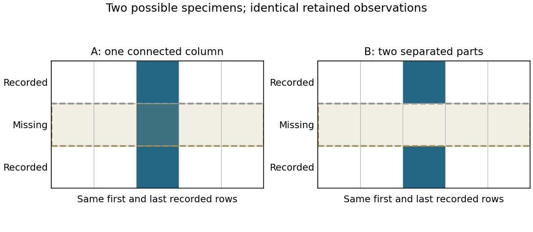
Original binary-volume counterexample: the two possible middle layers give identical retained sections but different connectivity
. Details. Lateral position jitter is the fluctuating in-plane displacement of successive acquired images relative to a chosen reference. In serial block-face scanning electron microscopy, it can displace corresponding features between block faces even when the cutting increment is perfectly regular. A simple image registration model iswhere is the ideal image of the current face and is its lateral shift. The specimen itself changes between faces, so not every apparent shift is instrumental motion.
A primary apparatus study estimated inter-image displacement from cross-correlation peaks in several subregions. Its Figure4 central cluster had standard deviations of and along the two axes; outliers and changing specimen patterns required interpretation.[ref]
Serial Block-Face Scanning Electron Microscopy to Reconstruct Three-Dimensional Tissue Nanostructure by Winfried Denk and Heinz Horstmann. Results, registration paragraph; Figure4 and caption; Materials and Methods, Data analysis
For an original one-axis example, take measured frame offsets pixels at pixel pitch . The offsets are and their root mean square about zero isThe successive differences are , whose root mean square is . These are different statistics. For independent equal-variance frame offsets, the theoretical difference variance is ; correlation or drift changes that relation. Specify the reference, detrending and normalization when reporting jitter. Image registration can estimate a correction but does not prove that all residual motion or specimen deformation has been removed.
A special semimartingale is a semimartingale admitting a decompositionwith a zero-starting local martingale and a zero-starting predictable finite-variation process. Predictability of the finite-variation term is the additional requirement. With these starting conventions, this canonical decomposition is unique.
For a rate- Poisson process , the decomposition is . The compensated part is a martingale, and the drift is deterministic, hence predictable. Although itself has finite-variation paths, assigning all of it to the finite-variation term would not give the canonical predictable decomposition.
Uniqueness follows because the difference between two such decompositions is both a local martingale and a predictable finite-variation process starting at zero, which must vanish. Predictability cannot be omitted from that argument: is a nonconstant local martingale with finite-variation paths on compact intervals.
A thermal-product input-distribution check tests whether the probability model used for a nonlinear thermal correction describes the available temperature and material information. In , with coefficient difference and temperature offset , the uncertainty depends on their joint behaviour, not just on two separately quoted standard uncertainties.
Start with the physical inputs: which thermometer calibration is shared, how coefficient estimates were obtained, and whether either quantity was inferred using the other. Translate those relationships into a joint distribution or an explicit dependence model. JCGM 101 distinguishes assigning input distributions from propagating them through a measurement model; numerical sampling cannot supply missing physical information.[ref]
An original counterexample shows why zero covariance is insufficient for the independent-input formula. Let be standard normal and defineBoth inputs have zero mean, with variances and , and their covariance is zero because the required Gaussian odd moments vanish. They are nevertheless dependent: is determined by .
Their product has zero mean and varianceusing Gaussian moments , , . Independence would instead give . With , and , the resulting standard deviation is about 22.36 nm rather than 10 nm. This is a deliberately constructed probability example, not a claim about typical thermometers.
Thermal-product dependence beyond covariance matters because higher moments enter the product variance. A multivariate normal distribution is a particular joint model whose moments are determined by its means and covariance; arbitrary inputs sharing those same summaries need not behave identically.
Check units, support, marginal shapes and dependence before simulation. Compare exact or limiting cases with a Monte Carlo method, and retain a sensitivity analysis for plausible alternative input models. The GUM's first-order rule requires higher-order treatment when nonlinearity matters.[ref] A small simulation error measures numerical precision conditional on the model, not proof that the model is physically correct.
A scheme point is a point of the underlying topological space of a scheme, together with the local algebra supplied by its structure sheaf. On an affine scheme , points correspond to prime ideals , and the local ring at the point is . Closed points correspond to maximal ideals; schemes also have nonclosed points.
For , each prime number gives a closed point with residue field . The prime ideal is a nonclosed generic point with residue field . Its closure is the whole spectrum, so it records the common generic arithmetic rather than one reduction modulo a prime.
More generally, the point for is a specialization of the point for exactly when . Thus incidence in the prime-ideal ordering becomes topology. Treating every scheme point as an ordinary coordinate tuple would discard this generic and specialization information.
KLT orthogonality states that vectors built from different solutions of the scattering equations are orthogonal under the field-theory KLT bilinear form. For generic massless kinematics, label the solutions by . Define the Parke-Taylor factor for a cyclic ordering byLet evaluate this factor at solution in ordering and in ordering . If is the KLT momentum kernel, thenwith nonzero diagonal pairings generically.[ref]
Scattering Equations and KLT Orthogonality by Freddy Cachazo and others. Section 5.2, equations (29)–(34), Proposition 2
The pairing is bilinear, without complex conjugation; it is not an ordinary positive Hermitian inner product. At four points there is only one solution, so the off-diagonal statement is vacuous. At five points two solutions yield two vanishing cross-pairings. The proof relates the pairing to a generalized scattering-equation Jacobian whose rank drops from to for distinct solutions, forcing the relevant minor to vanish. This eliminates mixed-solution terms when combining gauge-theory amplitudes into gravitational amplitudes.[ref]
Scattering Equations and KLT Orthogonality by Freddy Cachazo and others. Section 5.1, Proposition 1; Sections 5.2 and 6.1
Beam root rotational compliance is the incremental rotation of a beam's attachment relative to its supporting base per increment of applied root torque. For a linear rotational restraint with stiffness ,The angle is measured in radians, so the compliance can be reported in . The root's transverse position is held fixed in this model. The rotational spring boundary condition for a beam implements this finite restraint; a clamped boundary condition is the zero-compliance limit. End moments and section rotations are conjugate quantities in beam virtual work.[ref]
For an original static derivation, apply a transverse tip force to a beam of length and constant beam flexural rigidity . The root moment has magnitude , giving . In the small-angle approximation, root rotation contributes to tip displacement. Bending relative to that rotated attachment gives the usual cantilever contribution, soThis derivation assumes a linear elastic beam, no root translation and an effectively rigid supporting base. The second term is fixture motion rather than a change in material Young's modulus.
For stipulated , , and , the root rotates through radian. Root motion contributes , while bending contributes . Attributing the entire to a perfectly clamped beam would infer instead of the stipulated value six.
A proposed measurement uses a known force and lever arm to apply a root moment, with optical markers on the attachment and on the supporting base to measure their relative angle. A separate displacement channel can detect unwanted root translation. Fit the small-load slope of angle against moment; using only the beam-tip displacement would mix attachment rotation with beam bending. Load reversal tests whether one linear compliance adequately describes the fixture or whether backlash and hysteresis require another model.
The RNA polymerase bridge helix is an alpha helix spanning the active site region of RNA polymerase. In RNA polymerase II, it lies near the template DNA and growing RNA, where conformational changes can alter the space available for template positioning during transcription.[ref]
Researchers soaked transcription elongation complex crystals with alpha-amanitin. The trapped structure showed the entering DNA base above a shifted RNA polymerase bridge helix, with the usual templating position obstructed. The authors interpreted the arrangement as a possible intermediate in movement along DNA.[ref]
Structural basis of transcription inhibition by alpha-amanitin and implications for RNA polymerase II translocation by Florian Brueckner and Patrick Cramer. Abstract: inhibitor soaking and proposed translocation intermediate
The useful connection is between local protein geometry and which DNA base can be presented to the catalytic machinery. Successive addition cycles require that relationship to change while sequence order remains intact. A trapped conformation is evidence about an accessible arrangement; establishing its timing and contribution to normal movement also requires kinetic measurements. The helix is part of the coupled enzyme, rather than an independently operating motor.
The RNA polymerase trigger loop is a mobile protein element near the active site of multisubunit RNA polymerase. In RNA polymerase II, it can close beneath a correctly positioned incoming nucleoside triphosphate and form contacts with its base, sugar and phosphate groups. Its movement links recognition of the substrate with efficient phosphodiester bond formation during transcription.[ref]
Structural basis of transcription: role of the trigger loop in substrate specificity and catalysis by Dong Wang and others. Abstract and Figures 1–2: substrate contacts and alternative loop conformations
The 2006 structural study compared transcribing complexes with different bound nucleotides. A correct substrate in the addition site was associated with a closed conformation and an extensive interaction network. This gave a physical explanation for why merely entering the active-site region is not sufficient for efficient incorporation: the substrate must also support a productive arrangement of the surrounding polymerase.[ref]
Structural basis of transcription: role of the trigger loop in substrate specificity and catalysis by Dong Wang and others. Figures 1–2, addition/entry-site nucleotide complexes and trigger-loop positions
For an illuminating comparison, imagine two nucleotides that bind detectably but support loop closure with different probabilities. Equal binding abundance would not imply equal incorporation rates, because productive positioning contributes a further step. This is a schematic kinetic argument, not a measurement of a particular pair of rate constants.
The adjacent RNA polymerase bridge helix and the RNA polymerase trigger loop are distinct structural elements. A proposed catalytic role for a loop residue must also be distinguished from what is directly observed in a crystal: geometry can suggest a chemical mechanism, while mutagenesis and kinetics test its consequences.
The concentration dependence of RNA melting is the change of an RNA melting temperature or population curve with total strand molar concentration, while other solution conditions are held fixed. It helps distinguish intramolecular RNA hairpin melting from association of separate strands, provided the system reaches chemical equilibrium.
For an ideal unimolecular folded-to-unfolded transition, , the equilibrium constant is . Multiplying both populations by the same amount leaves their ratio unchanged: the two-state RNA melting model has no total-concentration term. By contrast, consider self-complementary RNA duplex melting, with association . Let count strands and let denote the reference molar concentration of the standard state. The dimensionless association equilibrium constant isAt the midpoint defined by half the strands belonging to duplexes, and , giving . This factor follows from strand counting; a different reaction or midpoint convention requires its own derivation.
An original ideal calculation assumes constant association enthalpy and a midpoint at . Increasing strand molar concentration tenfold givesor approximately . Here is the molar gas constant. Greater strand availability favors association, so more heating is needed to reach the same strand-based midpoint.
Experimentally, one records RNA optical melting curves at several strand molar concentrations, with matched solvent conditions. A tetraloop study found concentration-independent transitions over approximately a 50-fold range, supporting intramolecular stem–loop formation.[ref]
Thermodynamic characterization of naturally occurring RNA tetraloops by Justin P. Sheehy and others. Materials and Methods, Optical melting experiments and thermodynamics.
This test is conditional on reversibility: a kinetically trapped association can fail to show the expected equilibrium concentration response.An RNA melting relaxation time characterizes how quickly a perturbed RNA population approaches its new equilibrium. It belongs to a specified kinetic model, temperature, solution and measured signal. It is not an RNA melting temperature or, in general, the mean waiting time for an individual unfolding event.
For a reversible two-state RNA melting model, let be the first-order unfolding rate constant and the refolding rate constant. The unfolded fraction obeysAt fixed temperature,Both directions contribute to the return to equilibrium. For original stipulated values and , and . The mean lifetime of an isolated folded state in this model is , which differs from the observed population exponential decay time.
A temperature jump shifts populations rapidly enough to reveal the subsequent motion. A primary study used 4-ns heating pulses, a 12-μm sample path and time-resolved infrared spectroscopy to follow melting and refolding of a UACG-containing RNA hairpin. Thin-cell cooling enabled direct observation of the return process. Its loop is UACG, not a UUCG tetraloop.[ref]
Measuring RNA UNCG Tetraloop Refolding Dynamics Using Temperature-Jump/Drop Infrared Spectroscopy by C. P. Howe and others. Printed pp.9171–9172, sequence and pump/probe apparatus; Abstract, melting and refolding dynamics.
An RNA relaxation instrument-response correction may be needed if heating, detector response or cooling occur on comparable timescales. A changing sample temperature changes the equilibrium target during the measurement, invalidating a constant-temperature fit across the whole trace. Multiple kinetic states can also produce several decay components. One fitted exponential should therefore be identified as a model-dependent observed relaxation, rather than automatically assigned to a unique molecular step.
RNA baseline extrapolation continues a fitted folded-state or unfolded-state RNA melting baseline from its observed temperature range into the transition region. It is necessary when estimating populations from RNA optical melting, because both hypothetical pure-state signals are needed at temperatures where the measured sample contains a mixture.
For a linear folded baseline, choose a reference and writeThe reference merely changes parameterization. An original fit with , and predicts 0.420 at and 0.450 at . The first prediction might interpolate within measured data; the second extrapolates if all folded-state observations were below .
The inferred population depends on that continuation. At , suppose measured absorbance is 0.600 and the unfolded RNA melting baseline is 0.700. The linear folded-baseline prediction givesIf the actual pure folded-state response there were 0.490, the same optical-mixture equation would instead give . A good fit in a limited low-temperature region does not rule out curvature beyond it.
RNA baseline prediction covariance is important even within the chosen linear model. With ,For stipulated independent fit parameters and , the prediction's standard uncertainty rises from 0.002 at to approximately 0.0102 at . This is uncertainty propagation for estimated parameters; it does not include unmodeled curvature.[ref]
Evaluation of measurement data — Guide to the expression of uncertainty in measurement by JCGM. §§5.1–5.2, linear sensitivities and correlated inputs.
Optical-melting experiments fit signal curves to infer thermodynamics.[ref]
Thermodynamic characterization of naturally occurring RNA tetraloops by Justin P. Sheehy and others. Materials and Methods, individual-curve thermodynamic fitting.
Report which regions constrain each RNA melting baseline, inspect residuals and compare plausible baseline forms. Confidence in the fitted parameters and confidence in the functional form are different parts of the inference.An RNA isostericity matrix organizes the geometric compatibility of base pairs in a specified RNA base-pair geometry family. Its purpose is to help identify substitutions that approximately preserve the arrangement of the attached backbones. It is not a table of base-pair free energies or a substitution-probability matrix.[ref]
The non-Watson-Crick base pairs and their associated isostericity matrices by Neocles B. Leontis and others. Isostericity matrices, printed p. 3525, Tables 3–5
The layout must be checked. In the 2002 classification, a family-specific four-by-four table uses one nucleobase identity for each axis; each entry locates an ordered base combination and assigns it to an isosteric subgroup where supported. Parentheses distinguish modeled contacts from observed ones. In later quantitative comparisons, rows and columns can instead both label complete base-pair exemplars, with entries giving their geometric discrepancy. These are different uses of a matrix layout.[ref]
For the canonical cis Watson–Crick family, A–U, U–A, G–C and C–G belong to subgroup I1. As an original teaching encoding, label those four pair types and put when the classification regards as mutually compatible. Their restricted block isThis binary comparison block is not a reproduction of the published identity-grid layout. It encodes six distinct unordered substitutions, with diagonal entries representing self-comparison. It does not assert equal hydrogen bond counts, equal folding stability or unrestricted interchange in every RNA motif.[ref]
The 2009 quantitative study uses the RNA IsoDiscrepancy Index to distinguish isosteric, near-isosteric and more dissimilar exemplars. In that study, values at most2.0are classified as isosteric and values above2.0through3.3as near-isosteric. These cutoffs accompany the authors' structural comparison method; they are not universal energy thresholds.[ref]
Frequency and isostericity of RNA base pairs by Jesse Stombaugh and others. Results, Figure 2 and Table 3
When applying a matrix, state the geometric family, order of the two bases, structural exemplars and meaning of each entry. An unobserved entry is not proof that a contact is impossible. Likewise, a compatible substitution is a geometric hypothesis to test in its structural context, not a guarantee of unchanged biological function.
The RNA IsoDiscrepancy Index, abbreviated IDI, is a numerical measure of how two base pairs differ in the geometry relevant to their attached backbones. Lower values indicate closer RNA base-pair isostericity. Jesse Stombaugh, Craig L. Zirbel, Eric Westhof and Neocles B. Leontis introduced it to make comparisons more quantitative than assigning pairs only to broad geometric families.[ref]
Frequency and isostericity of RNA base pairs by Jesse Stombaugh and others. The IsoDiscrepancy Index, Definition
The comparison considers the separation of the ribose atoms and the relative positions and orientations of the bases at their glycosidic bonds. The attachment nitrogen is N1 for a pyrimidine and N9 for a purine. Thus matching the distance between two sugar attachment points alone does not establish matching base orientation. The published construction handles in-plane alignment and comparisons requiring an out-of-plane flip separately.[ref]
Frequency and isostericity of RNA base pairs by Jesse Stombaugh and others. Definition, geometric criteria and Cases 1–2
IDI has units of ångströms, not a dimensionless probability scale. In the in-plane case, the method weights an orientation angle by a 2-ångström length scale. An original illustration of that rotation term isThis is one weighted rotation contribution, not the complete IDI formula. Translation, separation and the paired orientation comparisons also matter. Expressing an angle in radians is essential to this length interpretation.[ref]
Frequency and isostericity of RNA base pairs by Jesse Stombaugh and others. Definition, interpretation of the coefficient multiplying the in-plane rotation angle
The authors calibrated their classification using structural distributions: IDI at most 2.0 ångströms is isosteric, above 2.0 through 3.3 ångströms is near-isosteric, and larger values are more dissimilar. These are the study's method-specific cutoffs. A chosen score of 1.8 therefore falls in its first category, whereas 2.6 falls in its second; neither is an energy or a probability.[ref]
Frequency and isostericity of RNA base pairs by Jesse Stombaugh and others. Validation of the IDI, Figure 2 and Table 3
Interchanging the two structures being compared leaves the discrepancy unchanged; reversing the nucleotide order within only one base pair is a different operation. An RNA isostericity matrix can display such comparisons, but sequence context and model quality still affect interpretation. A geometrically plausible substitution is a structural hypothesis, not a guarantee of unchanged folding stability or molecular recognition.
Pinned article: Introduction to the OurBigBook Project
Welcome to the OurBigBook Project! Our goal is to create the perfect publishing platform for STEM subjects, and get university-level students to write the best free STEM tutorials ever.
Everyone is welcome to create an account and play with the site: ourbigbook.com/go/register. We belive that students themselves can write amazing tutorials, but teachers are welcome too. You can write about anything you want, it doesn't have to be STEM or even educational. Silly test content is very welcome and you won't be penalized in any way. Just keep it legal!
Intro to OurBigBook
. Source. We have two killer features:
- topics: topics group articles by different users with the same title, e.g. here is the topic for the "Fundamental Theorem of Calculus" ourbigbook.com/go/topic/fundamental-theorem-of-calculusArticles of different users are sorted by upvote within each article page. This feature is a bit like:
- a Wikipedia where each user can have their own version of each article
- a Q&A website like Stack Overflow, where multiple people can give their views on a given topic, and the best ones are sorted by upvote. Except you don't need to wait for someone to ask first, and any topic goes, no matter how narrow or broad
This feature makes it possible for readers to find better explanations of any topic created by other writers. And it allows writers to create an explanation in a place that readers might actually find it.
Figure 1. Screenshot of the "Derivative" topic page. View it live at: ourbigbook.com/go/topic/derivativeVideo 2. OurBigBook Web topics demo. Source. - local editing: you can store all your personal knowledge base content locally in a plaintext markup format that can be edited locally and published either:This way you can be sure that even if OurBigBook.com were to go down one day (which we have no plans to do as it is quite cheap to host!), your content will still be perfectly readable as a static site.
- to OurBigBook.com to get awesome multi-user features like topics and likes
- as HTML files to a static website, which you can host yourself for free on many external providers like GitHub Pages, and remain in full control

Figure 2. You can publish local OurBigBook lightweight markup files to either OurBigBook.com or as a static website.
Figure 3. Visual Studio Code extension installation.
Figure 5. . You can also edit articles on the Web editor without installing anything locally. Video 3. Edit locally and publish demo. Source. This shows editing OurBigBook Markup and publishing it using the Visual Studio Code extension. 
- Infinitely deep tables of contents:



All our software is open source and hosted at: github.com/ourbigbook/ourbigbook
Further documentation can be found at: docs.ourbigbook.com
Feel free to reach our to us for any help or suggestions: docs.ourbigbook.com/#contact