Topics (384k) Articles (398k) Users (410) Discussions (242) Comments (383) Files (13k) New article

A 2D IR response-factor validation mixture has independently established information about the spectral components of interest and is measured to test a response model under specified conditions. It tests 2D IR response-factor transferability rather than merely reproducing the same fit that supplied an unknown population.
In the positive-component model , , the 2D IR response-factor ratio predictsFor , independently known fractions predict ratios . Testing several fractions probes more of the response curve than one agreement at a single composition.
An original noiseless example exposes a background error. Suppose the actual measured components areIgnoring the additive terms and inferring a response ratio separately from each mixture givesAt , the results are approximately . Their composition dependence contradicts a single uncorrected response ratio even without measurement noise. Subtracting the stipulated background from each channel recovers the common value in this constructed model.
Independent composition information must also concern the quantity used in the model. A prepared mole fraction is not automatically the excited-state population fraction if the components absorb or are excited differently. Sample preparation, spectral assignment and the response model together determine whether a mixture is an appropriate validation reference.
A useful controlled comparison retains pulse spectrum, polarization, 2D IR waiting time, phase convention and amplitude-fitting rule, then changes the condition whose transferability is being tested. Blank measurements and mixtures not used to estimate provide distinct checks. The primary response theory includes pathway-dependent transition-dipole products and relaxation factors, motivating this care with the selected observable.[ref]
Composition and background estimates carry measurement uncertainty. The uncertainty analysis should include shared inputs and covariance, rather than interpreting every departure from the curve as a new molecular mechanism.[ref]
Evaluation of measurement data — Guide to the expression of uncertainty in measurement by JCGM. Sections 5.1–5.2, sensitivity coefficients and correlated inputs
A nested wringing-repeatability study separates variation between independently prepared gauge block wringings from readout scatter within one unchanged wring. Repeating a detector reading many times does not sample the contact variability introduced by separating and rejoining the surfaces.
For wrings with readings each, an original balanced random effect model iswhere independent wring effects have variance and independent readout errors have variance . Assume stable conditions and independence between those levels. One-way analysis of variance givesThus estimates readout variance and estimates the between-wring variance in this model. A negative variance estimate reflects sampling variability or model limitations, not a physically negative contact variance.
For a small invented data set, duplicate readings in nm relative to an arbitrary reference are , and . Wring means are ; and , so the method-of-moments between-wring variance is . These are arithmetic examples, not a recommended sample size or a NIST calibration result.
For the overall mean of the balanced study,With stipulated , , five wrings and four readings per wring, its standard deviation is . Increasing to forty readings on the same five wrings lowers it only to about 2.69 nm. Fifty wrings with four readings each would instead give about 0.86 nm, if the same model and stable preparation remain valid.
A shared reference or persistent preparation contribution does not disappear under either averaging rule. An independent common uncertainty adds to the displayed variance. This connects the nested study with the wringing-film covariance model and the gauge-block reference uncertainty floor.
NIST's handbook documents contact-layer dependence on preparation and time, including evolution after thermal equilibration.[ref] Record rewringing events, timestamps and surface preparation; use appropriate controls for drift and damage. A nested contact-study allocation should balance new wrings against repeat readings, rather than treating every reading as an independent contact experiment.
Unit-intensity Gaussian space-time white noise is a random distribution specified through its integrals against square-integrable deterministic functions. Write that integral as . The family is centered and jointly Gaussian, linear in , and satisfiesFormally one writes , but is not an ordinary pointwise random variable. The integrated definition gives the delta notation a precise meaning.[ref]
An Introduction to Stochastic PDEs by Martin Hairer. Section 2.3.1, white-noise covariance; Example 4.63, equation 4.17 and its space-time extension
For a space-time region of finite volume , define . Then , and disjoint regions have independent noise integrals. The average over the region has a different scaling:Shrinking the averaging region increases the variance of the average. This prevents taking a finite-variance pointwise limit.
For an independent numerical example in one space dimension, a rectangular cell has volume . Its noise average can be sampled as with . In normalized coordinates, and give standard deviation about . Giving every refined grid cell the same variance would change the continuum noise model.
Convolving space-time white noise with a heat kernel produces the random forcing contribution to a stochastic heat equation. Whether that smoothed field has pointwise values depends on dimension and the smoothing operator; the noise definition alone does not imply a continuous signal.
Inverse-variance weighting combines estimates of the same quantity by giving a more precise estimate a larger weight. Suppose are independent, unbiased estimators of , with known variances . For normalized weights,The inverse is taken after squaring the standard uncertainty: twice the standard uncertainty gives one quarter as much weight. The corresponding weighted least squares criterion is ; differentiating it with respect to gives the same weighted arithmetic mean.[ref]
The optimality statement is precise. Any linear unbiased estimator requires . By the Cauchy-Schwarz inequality,Equality holds for the displayed weights. Thus they minimize variance among linear unbiased combinations under these assumptions; a normal distribution is not needed for that proof.
For an original example, combine observed values 10 and 14 with standard uncertainties 1 and 2 in the same units. The normalized weights are and , giving estimate , variance and standard uncertainty approximately . Equal weights give 12 and standard uncertainty .
Correlated errors change the problem. A contribution common to every reading survives every weighting whose coefficients sum to one; precision limits of weighting correlated repeats derives the resulting floor. More generally, use the full covariance matrix and generalized least squares rather than treating correlated readings as independent.[ref]
Guide to the expression of uncertainty in measurement by JCGM. §5.2.2, equation13, and §5.2.4, common inputs
Uncertainty in estimated inverse-variance weights is another limitation: variances estimated from the same data are not fixed known quantities, and an accidentally tiny estimated variance does not justify arbitrary confidence.Coupled L2 regularization adds a quadratic parameter penalty to the objective function and sends its gradient through the same optimizer update as the data gradient. With coefficient , defineSince the gradient of the squared Euclidean norm divided by two is , a supplied data gradient becomesThe factor fixes the convention: a penalty written as instead contributes .
For plain gradient descent, this substitution givesIt is therefore equivalent to decoupled weight decay with the matched coefficient in this particular update. The equivalence need not survive coordinate-dependent processing of the gradient.[ref]
Decoupled Weight Decay Regularization by Ilya Loshchilov and Frank Hutter. Version3, section2, propositions1–2 and AppendixA
For an original fixed-scaling example, let , , , and diagonal matrix . Applying to the whole coupled gradient givesThe same quadratic penalty produces unequal coordinate shrinkage after this scaling. Uniform decoupled weight decay would instead give . The example isolates a fixed scaling operation, rather than claiming to simulate a complete adaptive gradient method.
Coupling can also change the optimizer state. For example, a momentum buffer formed from stores contributions from along with the data gradient. If an adaptive accumulator uses squared gradient entries, it receives , including a cross term . Subsequent updates can therefore differ even when the next data gradient is the same. State both the penalty convention and the optimizer's gradient-processing rule when describing an L2 setting.
Decoupled weight decay applies a parameter-shrinkage contribution separately from the optimizer's processing of the data gradient. Write for the processed data-gradient direction, including any algorithm-specific optimizer state. Using the coefficient convention documented for PyTorch AdamW,The shrinkage term uses the pre-update parameter and is not inserted into the gradient moments.[ref]
AdamW in the PyTorch documentation. PyTorch2.15, algorithm: separate parameter-decay line before the adaptive update
This differs from coupled L2 regularization, which processes as a single gradient input. Decoupled weight decay was introduced for adaptive optimization in the AdamW work; the original paper also writes decay coefficients with the learning-rate factor absorbed differently, so its coefficient must be translated before comparing equations.[ref]
Decoupled Weight Decay Regularization by Ilya Loshchilov and Frank Hutter. Version3, section2 and Algorithm2
An original limiting case isolates the shrinkage. Suppose the processed direction is zero at every step and are constant. Repeated substitution givesWith , and , one update gives 0.98 and 50 updates give approximately 0.36417. For varying learning rates, the corresponding factor isThus the same numerical decay coefficient can have a different accumulated effect under a different learning rate schedule. In this zero-direction model, gives sign-preserving shrinkage; other factors have different behaviour.
The update order is also part of the definition. For , , and , the stated formula gives . Applying shrinkage after first taking the gradient step would instead give . Both operations may be described informally as decay plus a step, but they are different recurrences. An optimization checkpoint must retain the relevant state and settings to reproduce the chosen one.
Reciprocal size-ratio ambiguity in centred Gaussian overlap means that one beat-efficiency measurement cannot distinguish a beam that is too wide from one that is reciprocally too narrow. Under the matched-curvature, matched-polarization model of waist-size mismatch in optical heterodyne mode matching,Solving for the ratio at gives two roots,For an original measured efficiency , the ratios are and . With a known reference radius , the other beam could have radius or . This is an exact two-branch ambiguity, even for a noiseless measurement.
Put . Then , an even function of the signed logarithmic mismatch. Close to matching, , so the first-order response to a small signed mismatch vanishes. Beat efficiency alone is both sign-ambiguous and weakly sensitive near its maximum.
A branch selection by a controlled beam-radius change can distinguish the two possibilities if other optical properties stay fixed. Increasing by changes the ratio to , increasing efficiency to about ; it changes to , decreasing efficiency to about . This is a conditional diagnostic: a lens adjustment that also changes curvature or displacement need not follow this one-parameter curve.
NIST used matched optical modes and polarization in the physical heterodyne calibration setup.[ref]
Frequency response metrology for high-speed optical receivers by Paul D. Hale and others. PDF p. 1, Heterodyne measurements
Independent beam profiling at the receiving plane supplies the missing radius information directly; power balancing alone does not resolve this ambiguity.Vibrational spectral diffusion is the evolution of a molecular vibrational transition frequency as its surroundings or configuration fluctuate. It concerns frequency memory within a vibrational response, whereas vibrational relaxation concerns loss or redistribution of vibrational excitation. Their characteristic times need not coincide.
In two-dimensional infrared spectroscopy, an initial frequency label is followed by an independently varied 2D IR waiting time and a later frequency-sensitive readout. The vibrational frequency-frequency correlation function models the relation between those earlier and later frequencies, while a 2D IR center-line slope summarizes part of the measured spectral geometry under specified response assumptions.[ref]
Frequency-frequency correlation functions and apodization in two-dimensional infrared vibrational echo spectroscopy: A new approach by Kyungwon Kwak and others. Introduction and §II.A, frequency labeling, population interval and correlation-function model
An original two-state vibrational frequency memory model has equally populated environments with spectroscopic frequencies and . Suppose switching in either direction follows a continuous-time Markov chain with rate . With a sign variable , the probability of a flip during is ; each flip reverses its frequency deviation. Hence the normalized sign memory satisfiesThe memory time is , not the mean residence time in either state. Returning to the initial state contributes to the measured memory, so these two time scales describe different events.
For stipulated transitions at 1000 and with , the mean is , the variance is and the memory time is 2 ps. At 2 ps the correlation is . The probability of occupying the initial environment is , including trajectories with an even number of switches.
If an independent vibrational population in this illustrative model decays with lifetime 10 ps, its surviving fraction at 2 ps is , while normalized frequency memory is only 0.368. This explicitly separates population survival from frequency decorrelation. These are model values, not measured solvent or vibrational constants.
The model uses spectroscopic wavenumber, not angular frequency. Converting to an angular-frequency correlation multiplies by when the speed of light uses compatible length units. Mixing these conventions changes the fluctuation amplitude without changing the switching time.
To test the interpretation, acquire spectra at several waiting times, characterize pulse timing and phase, and assess overlap, population decay and instrument response. A decaying spectral statistic can constrain frequency fluctuations, but the same observed decay may fit more than one microscopic environment model. The two-state calculation is a reusable mechanism example, not a universal explanation of spectral diffusion.
A recognition network is a learned mapping from observed data to parameters of an approximate posterior distribution over latent variables. In a variational autoencoder, it specifies , while the generative decoder specifies the opposite conditional direction . The recognition network supports amortized inference; it need not coincide with the exact posterior of the learned generative model.[ref]
Auto-Encoding Variational Bayes by Diederik P. Kingma and Max Welling. §3 and Appendix C, neural-network recognition model
For a scalar Gaussian recognition law, the neural network can output a mean and log variance . Thenwhere is parameter-independent noise. Exponentiating the log variance ensures a positive variance, and the factor converts it to the standard deviation used in Gaussian reparameterization.[ref]
Auto-Encoding Variational Bayes by Diederik P. Kingma and Max Welling. Appendix C.2, Gaussian output mean and log variance
For an original calculation, suppose one input gives and . The recognition variance is4 and its standard deviation is2. A noise draw gives , while the posterior mean supplied by the same network remains1. Confusing log variance with log standard deviation would instead produce the wrong scale.
A deterministic network evaluation and a random latent sample are distinct steps. Re-evaluating the same fixed network on the same input returns the same distribution parameters; new noise draws can still yield different values. Returning only the mean omits the uncertainty represented by that distribution. Its adequacy must be assessed against the intended inference problem, not inferred merely from the fact that it outputs a positive variance.
A generative decoder maps a latent variable to the parameters of a conditional observation probability distribution, commonly written . In a variational autoencoder, a neural network can supply those parameters. The conditional law, including its observation noise and support, is part of the model; the decoder need not return one deterministic reconstructed observation.[ref]
Stochastic Backpropagation and Approximate Inference in Deep Generative Models by Danilo Jimenez Rezende and others. §2, visible-layer distribution and generative transformations
For a concrete binary example, suppose a decoder specifies two conditionally independent Bernoulli distributions with probabilities and . ThenIf a chosen latent value gives , the conditional probability of is , and its negative log likelihood is approximately . The vector is a vector of probabilities, not itself a binary sample. A model for continuous observations would need a different conditional distribution.[ref]
Auto-Encoding Variational Bayes by Diederik P. Kingma and Max Welling. Appendix C.1–C.2, Bernoulli and Gaussian observation models
Generation draws a latent value from the prior and then draws from the decoder's conditional law. Averaging over latent values givesConditional independence of output components at fixed need not imply independence after this marginalization, because the same latent variable can influence several components. The recognition network runs in the other direction for inference; it is not an algebraic inverse of the generative decoder.
The Casimir effect is a force associated with the change in electromagnetic field fluctuations produced by material boundaries. For ideal perfectly conducting parallel plates separated by at zero temperature, the attractive pressure isReal measurements require finite-conductivity, temperature and geometric corrections. A classic experiment used a torsion-pendulum electromechanical system to measure the force between nearby conducting surfaces. The experimental comparison concerns the force difference produced by a specified geometry; it does not make an arbitrary absolute vacuum-energy offset observable.[ref]
A reference-sensitivity cancellation check determines whether a proposed comparison really removes the influence of a shared calibration reference. It checks the measurand, the reference's sensitivity coefficients and the range over which the claimed cancellation applies.
For estimates and , a contrast has local reference sensitivityIts first-order reference variance is . Checking the contrast directly and checking the full covariance propagation should agree. The GUM defines the sensitivities and retains correlations between inputs.[ref]
An original linear model is and . For , the sensitivity is . Recomputing the unchanged comparison with the assigned reference value increased by changes by . With reference standard uncertainty 20 nm, its contribution to this contrast is 0.4 nm. Treating the two uses of as independent would miss this suppression.
A useful computational check perturbs one shared input consistently in every place it occurs. Perturbing its occurrences independently tests a different model. Finite-perturbation reference sensitivity also reveals whether a derivative evaluated at one point adequately describes the actual uncertainty range.
Zero first derivative is weaker than exact invariance. For an illustrative nonlinear model, take and . The derivative of vanishes at , but a reference perturbation leaves a term . If is zero-mean normal with standard deviation , that term has mean and standard deviation . The first-order cancellation has not removed the nonlinear contribution.
With stipulated and , these are nm and about 1.41 nm. These are model coefficients, not measured comparator behaviour.
Finally, verify that the chosen contrast is the quantity the experiment intends to determine. Replacing by another combination solely to cancel a reference changes the question. Retain calibration lineage and independent checks on comparator response; NIST's physical uncertainty budget distinguishes the master history from comparison-process variability.[ref]
Pulse-energy bounds from tail duration and pedestal height convert independently justified constraints on low-level light into a bound on total laser pulse energy. Peak power and full width at half maximum alone do not constrain an arbitrarily long below-threshold tail, as unbounded pulse energy at fixed peak and FWHM demonstrates.
Consider a nonnegative isolated power profile with peak , one contiguous half-maximum interval of duration , and total support of duration at most . Suppose power outside that interval is at most . ThenThe lower bound uses the half-maximum condition within the interval. The upper bound fills that interval to and every permitted remaining instant to . These bounds assume the stated shape class; multiple half-maximum crossings require an explicit interval convention.
For an original , , and , they give . Suppose a calibrated measurement additionally determines core energy . The pulse-energy interval from incomplete tail measurements tightens towith the displayed product using watts and nanoseconds. Reducing the independently established tail duration to tightens the upper bound to without changing the measured peak or width.
A receiver with characterized low-level response and a sufficiently long acquisition window is needed to justify and . A trace that falls below a detector threshold establishes no later support cutoff by itself. NIST's pulse-energy calibration discussion separates temporal waveform measurement from background and leakage effects.[ref]
Calibration Service for Low-level Pulsed-Laser Radiometers at 1.06 µm: Pulse Energy and Peak Power by Rodney W. Leonhardt. §§3.4–3.5, transfer and reference standards; §7.2, Leakage Effect
The numerical bounds above are conditional mathematical examples, not specifications of that apparatus.A diamond knife uses a sharpened diamond edge to cut ultrathin sections in ultramicrotomy. The edge's geometry and condition affect the force applied to the specimen and the resulting section. JEOL describes its use for hard inorganic materials and for obtaining uniform sections from resin specimens.[ref]
The knife wedge angle is the angle between the blade faces. It differs from the knife clearance angle, which concerns how the blade is oriented relative to the freshly cut surface. Manufacturer descriptions include and knife families, with the lower-angle design promoted for reduced section compression and a higher-angle design discussed for hard materials.[ref]
Ultra diamond knives by DiATOME. ultra35° and ultra45° manufacturer descriptions; materials applications
For an original ideal symmetric wedge of included angle , the blade width a distance behind the apex isAt , this gives for and for . The wider ideal wedge has about 31% more material behind the edge at that distance. This illustrates a geometry tradeoff; it does not predict a 31% difference in cutting force or assert the exact profile of a commercial knife.
A useful materials experiment compares otherwise matched cuts while recording knife orientation, feed and specimen condition, then measures section dimensions and surface defects. A cut stripe that repeats at the same lateral position suggests an edge-related artifact worth checking. Diamond hardness alone does not guarantee an undamaged edge or an undistorted section.
Ultramicrotomy prepares extremely thin physical sections by advancing a specimen block through a controlled increment and cutting across it with an ultramicrotome. A diamond knife or suitable glass knife removes the section; collected sections can then be examined by transmission electron microscopy. The instrument's feed setting and the geometry of the recovered section are related quantities, but they need not be equal. JEOL explicitly notes dependence on specimen material and temperature.[ref]
Ultramicrotomy by JEOL. Definition and specimen-feed description; actual-thickness dependence on resin and environmental temperature
For a materials example, consider a polymer block containing an initially -long marked interval parallel to the cutting direction. Suppose the recovered section measures along that interval, with unchanged transverse width. Its section compression is . Under an explicitly ideal volume-conserving model, a nominal layer would then have recovered thicknessThe altered area and thickness give the same model volume: . This is an original diagnostic calculation, not a universal correction rule. Material loss, transverse strain or nonuniform deformation would invalidate the model.
A motivating preparation check therefore compares dimensions of recognizable material features before cutting and in the recovered section, while recording cutting direction and specimen conditions. An independent thickness measurement tests whether the feed is a good depth calibration. Image registration can align section images but cannot generally reverse unknown physical deformation. For serial-section electron microscopy, preserve section order and gaps in the image stack as well as the chosen image stack axis calibration.
An RNA melting log-odds plot graphs the natural logarithm of the unfolded-to-folded population ratio against reciprocal absolute temperature. For , let and . An ideal unimolecular two-state RNA melting model with temperature-independent unfolding enthalpy and entropy predictsThe slope is ; the intercept is . The equation is a testable model relation, not a reason to treat every transformed optical curve as linear.
For an original worked example, stipulate unfolded fractions 0.20 at and 0.50 at . Their log-odds are and 0, givingThe fitted enthalpy is approximately , and the model predicts at . A third measurement tests this prediction; two chosen points always determine a line.
The transformation also changes the noise. First-order uncertainty propagation gives an RNA melting log-odds uncertaintyFor the same small standard uncertainty , this gives at , but approximately 0.101 at . Thus equal uncertainty in population fractions produces heteroscedasticity in the transformed data; unweighted linear regression can overemphasize unreliable endpoint values. Exactly 0 or 1 cannot be transformed, and replacing them with arbitrary small offsets manufactures finite values.[ref]
Evaluation of measurement data — Guide to the expression of uncertainty in measurement by JCGM. §5, first-order sensitivity-coefficient method; derivatives here are for the stated transformation.
Fractions inferred from absorbance also inherit the fitted RNA melting baselines. Optical-melting thermodynamics depends on this modeling step.[ref]
Thermodynamic characterization of naturally occurring RNA tetraloops by Justin P. Sheehy and others. Materials and Methods, optical curves and thermodynamic fitting.
Curvature may motivate testing baseline errors, additional states or changes in heat capacity; the plot alone does not identify which explanation is correct.In a finite connected graph with unit edge electrical resistances, orient two edges and . The transfer current is the signed current through when one unit of electric current is injected at and removed at . If is the resulting vertex potential, Ohm's law giveswhere is the graph Laplacian. Potentials are determined up to an additive constant, which cancels in the difference.
On a unit-resistance triangle, injecting across one edge sends of the current along that edge and along the two-edge alternative path. Thus . The transfer-current theorem identifies this diagonal value with the probability that the edge belongs to a uniform spanning tree; exactly two of the triangle's three spanning trees contain it.
Electrical reciprocity makes the unit-resistance kernel symmetric. Reversing one edge orientation changes the appropriate sign, while the determinants giving joint tree-edge probabilities remain unchanged.[ref]
Local Characteristics, Entropy and Limit Theorems for Spanning Trees and Domino Tilings via Transfer-Impedances by Robert Burton and Robin Pemantle. Theorem1.1 and section4, transfer-impedance kernel and determinants
A tidal field describes the spatial variation of gravitational acceleration across an extended body. With , a small separation gives relative acceleration , where .
For a point mass, a radial separation is stretched at rate coefficient , while transverse separations are compressed with coefficient . The common acceleration can be removed by choosing a freely falling frame; these relative accelerations remain. This makes tides a probe of gravitational inhomogeneity rather than merely the strength of the local acceleration.
A third-order pulse correlation ghost is a correlation lobe generated by a real feature in the nonlinear gate, appearing at a delay where no separate input pulse need exist. It is a property of the measurement's cross-correlation, not automatically an optical prepulse or optical postpulse.
The optical pulse temporal contrast article derives the separated-replica model for , and nonoverlapping identical-shape pulses. In third-order intensity autocorrelation, the main, positive-delay and opposite-delay lobe weights are respectivelyThe physical delayed replica enters linearly when it meets the strong squared gate; its squared contribution to the gate creates the opposite-delay ghost. Lobe separation and negligible pulse overlap are assumptions of this simple decomposition.
For an original , the real postpulse has four percent of the main intensity and equal duration. Normalized to the correlation's main peak, its lobe is , while the ghost is . A feature at negative delay near that latter level does not establish a physical prepulse. The ghost-to-real-lobe ratio is exactly in this model. This ghost-level consistency test for a delayed pulse replica can check an interpretation, although an actual prepulse could also be present.
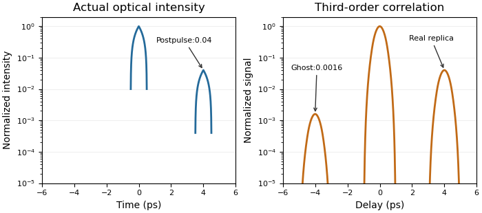
A real optical postpulse creates an opposite-delay ghost in an ideal third-order intensity autocorrelation
. Original compact triangular intensity profiles with a delayed replica at4ps and relative peak0.04. Direct numerical correlation produces the opposite-delay lobe near0.0016; the optical profile has no pulse there. Each panel is normalized to its own maximum. Source. Details.The historical correlator's inserted-etalon test supplies a controlled physical postpulse for checking the delay orientation.[ref]
A Single Shot 3rd Order Cross-Correlator for Pulse Contrast and Pulse Shape Measurements by J. Collier and others. printedp195, Results and Figure4
Independent changes to the replica strength, or a reference with known temporal structure, test the ghost interpretation. Overlapping pulses, unequal shapes and instrument backgrounds require a richer model. Pinned article: Introduction to the OurBigBook Project
Welcome to the OurBigBook Project! Our goal is to create the perfect publishing platform for STEM subjects, and get university-level students to write the best free STEM tutorials ever.
Everyone is welcome to create an account and play with the site: ourbigbook.com/go/register. We belive that students themselves can write amazing tutorials, but teachers are welcome too. You can write about anything you want, it doesn't have to be STEM or even educational. Silly test content is very welcome and you won't be penalized in any way. Just keep it legal!
Intro to OurBigBook
. Source. We have two killer features:
- topics: topics group articles by different users with the same title, e.g. here is the topic for the "Fundamental Theorem of Calculus" ourbigbook.com/go/topic/fundamental-theorem-of-calculusArticles of different users are sorted by upvote within each article page. This feature is a bit like:
- a Wikipedia where each user can have their own version of each article
- a Q&A website like Stack Overflow, where multiple people can give their views on a given topic, and the best ones are sorted by upvote. Except you don't need to wait for someone to ask first, and any topic goes, no matter how narrow or broad
This feature makes it possible for readers to find better explanations of any topic created by other writers. And it allows writers to create an explanation in a place that readers might actually find it.
Figure 1. Screenshot of the "Derivative" topic page. View it live at: ourbigbook.com/go/topic/derivativeVideo 2. OurBigBook Web topics demo. Source. - local editing: you can store all your personal knowledge base content locally in a plaintext markup format that can be edited locally and published either:This way you can be sure that even if OurBigBook.com were to go down one day (which we have no plans to do as it is quite cheap to host!), your content will still be perfectly readable as a static site.
- to OurBigBook.com to get awesome multi-user features like topics and likes
- as HTML files to a static website, which you can host yourself for free on many external providers like GitHub Pages, and remain in full control

Figure 2. You can publish local OurBigBook lightweight markup files to either OurBigBook.com or as a static website.
Figure 3. Visual Studio Code extension installation.
Figure 5. . You can also edit articles on the Web editor without installing anything locally. Video 3. Edit locally and publish demo. Source. This shows editing OurBigBook Markup and publishing it using the Visual Studio Code extension. 
- Infinitely deep tables of contents:



All our software is open source and hosted at: github.com/ourbigbook/ourbigbook
Further documentation can be found at: docs.ourbigbook.com
Feel free to reach our to us for any help or suggestions: docs.ourbigbook.com/#contact