The diffusion weighting b-value quantifies the encoding applied by a magnetic field gradient waveform in a diffusion measurement. For a refocused experiment in one spatial direction, defineHere $\gamma$ is the angular gyromagnetic ratio, in radians per second per tesla, and $G_{\mathrm{eff}}$ includes the sign reversal caused by the refocusing pulse. The echo time is $T$, with $q(T)=0$ for refocusing of stationary spins. Thus $q$ has units ${\mathrm{m}}^{-1}$ and $b$ has units $\mathrm{s}{\mathrm{m}}^{-2}$. The squared encoding history matters even though its final value is zero.^[ref]

For unrestricted, isotropic Gaussian diffusion with constant diffusion coefficient $D$, the otherwise matched signal ratio is $S/S_0=e^{-bD}$. Here $S_0$ uses the same pulse timing and detection conditions with the applied diffusion-encoding gradients removed. The diffusion weighting b-value describes the experiment's weighting; $D$ describes the assumed sample model.

For an original unit check, $1000\mathrm{s}\mathrm{m}{\mathrm{m}}^{-2}=10^9\mathrm{s}{\mathrm{m}}^{-2}$. With $D=10^{-9}{\mathrm{m}}^2{\mathrm{s}}^{-1}$, the ideal attenuation is $e^{-1}\approx 0.368$. Quoting a numerical $b$ without its units can therefore cause a millionfold scaling error.

The Stejskal-Tanner equation gives $b=(\gamma g\delta {)}^2(\Delta -\delta /3)$ for its equal rectangular pulses. More general waveforms require their own integral. For direction-dependent diffusion, a scalar $b$ alone cannot specify the complete directional encoding and response; a tensor description is needed.

Pulse width is the time separation of specified crossings on a pulse's leading and trailing edges. The threshold convention is essential when the edges are not instantaneous. Keysight's primary pulse-generator documentation uses the rising and next falling 50-percent crossings, and allows a duty-cycle setting as an alternative control.^[ref]

For low and high levels $V_L$ and $V_H$, define the fractional threshold as $V_L+a(V_H-V_L)$ with $0<a<1$. A positive pulse's width at that level is $\tau (a)=t_{\downarrow }(a)-t_{\uparrow }(a)$. The half-height convention is related to full width at half maximum for an isolated positive pulse above a defined baseline; it is not necessarily the duration of the flat top.

For an original asymmetric trapezoid, let a full linear rise take $t_r=2\mu \mathrm{s}$, the plateau last $H=8\mu \mathrm{s}$, and a full linear fall take $t_f=4\mu \mathrm{s}$. These ramp durations refer to the full low-to-high excursions, not the commonly quoted 10–90 percent rise interval. The crossing times giveThe 50-percent width is $11\mu \mathrm{s}$, while the first departure from the low level to final return lasts $14\mu \mathrm{s}$. At a 90-percent threshold the width is only $8.6\mu \mathrm{s}$. All describe the same waveform under different conventions.

For a repeating pulse train, duty cycle compares the specified width to the repetition period. Finite ramps mean that width times peak amplitude alone need not give the waveform integral or energy. Electrical loading and bandwidth also change the delivered crossings; the pulse generator setting must be checked at the actual load.

A measurement records both edges on an oscilloscope with a common level definition. Pulse-width uncertainty from correlated edge timing depends on $\mathrm{Var}(t_{\downarrow }-t_{\uparrow })$, including their covariance. A common trigger-time translation can cancel from width while remaining in absolute arrival time. Ringing with several crossings, hysteresis, negative pulses, or multiple peaks needs an explicit crossing-selection convention rather than an unspecified single duration.

Laser pulse energy is the radiant energy carried by one specified laser pulse across a measurement plane. For an isolated pulse whose total radiant power is $P(t)\ge 0$ and whose background is zero,Here $P$ is already integrated over the transverse beam area; it is not local irradiance. The unit of $U$ is the joule. Radiant exposure instead divides received energy by a receiving area, so a beam's $U$ alone does not specify the exposure at its centre. The radiant exposure of a Gaussian beam makes that spatial distinction quantitative.

The Gaussian pulse energy and peak power relation gives $P_{\mathrm{pk}}\simeq 0.939437U/\tau$ when $\tau$ is the power full width at half maximum. The pulse energy shape factor records pulse-shape dependence, while the Gaussian pulse field-envelope width is $\sqrt{2}$ times the power width.

For an original example, stipulate $U=0.50\mu \mathrm{J}$ and a Gaussian pulse power full width at half maximum $\tau =10\mathrm{ns}$. Then $P_{\mathrm{pk}}=46.97\mathrm{W}$. Stretching the same model pulse to $40\mathrm{ns}$ while keeping $U$ unchanged reduces its peak power to $11.74\mathrm{W}$. Both curves below integrate to the same energy; their peak heights and widths differ.

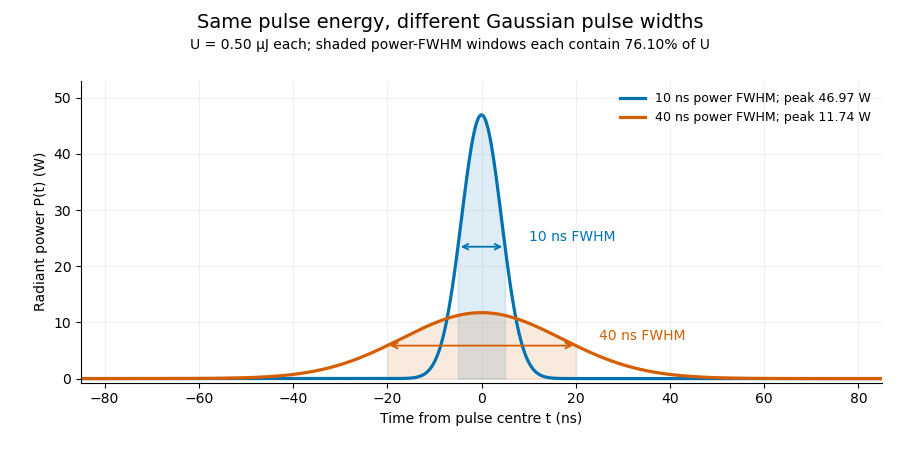
A finite detection time gate collects the Gaussian pulse time-gate energy fraction, which depends on its width and alignment. A centred gate as wide as the power full width at half maximum receives only $76.10\%$ of $U$, because Gaussian tails extend beyond it. For a $\tau$-wide gate, a Gaussian gate centring error of $\tau /2$ reduces capture to $49.07\%$.

The average power of a laser pulse train follows by counting complete pulses. If a long observation of duration $T$ contains $N$ pulses of energies $U_1,\dots ,U_N$, with negligible edge contributions and no continuous background,Here $f_{\mathrm{rep}}$ is the pulse repetition frequency, not the inverse pulse width. An average power readout constrains $\overline{U}$ when $f_{\mathrm{rep}}$ is known; it does not resolve pulse-to-pulse energy fluctuation. Identical, well-separated $0.50\mu \mathrm{J}$ pulses at $1.0\mathrm{MHz}$ give $0.50\mathrm{W}$ average power, even though the stipulated $10\mathrm{ns}$ pulses peak near $47\mathrm{W}$.

If a steady optical background is present, state whether the reported energy includes it. For pulse energy above a measured background $P_{\mathrm{bg}}$, the pulse energy baseline correction uses ${\int }_{\mathrm{gate}}[P(t)-P_{\mathrm{bg}}]dt$. Failing to subtract a constant background adds $P_{\mathrm{bg}}{T}_g$ to the inferred energy. This optical-background model is distinct from an offset introduced later by detector electronics.

Historical NIST equipment illustrates what the readouts measure. Its TC-24 reference absorbed the beam in a glass plate, sensed a plate temperature difference with thermocouples, and integrated the thermopile's electric potential difference during beam injection. Before/after readings enabled background subtraction and compensated thermal drift. Counting pulses converted total injected energy to mean pulse energy. The semiconductor pulse photodetector used an integrating amplifier; calibration related the peak output electric potential difference to pulse energy. That electrical peak did not by itself establish optical peak power.^[ref] Pulse energy measurement with a photodiode connects this kind of measurement to collected electric charge; validating the detector response under the actual pulse conditions remains part of that interpretation.

Pulse duration quantifies a pulse's temporal extent using a stated observable and width convention. A common optical convention is the full width at half maximum of the background-subtracted radiant power profile. The Ansys source documentation explicitly defines its PULSELENGTH parameter as the power-profile FWHM, rather than the width of the electric-field amplitude.^[ref]

For an original example, choose a triangular power pulseIts nonzero support extends from $-T$ to $T$, giving total support width $16\mathrm{ns}$. Its half-maximum crossings occur at $t=\pm T/2$, giving a power FWHM of only $8\mathrm{ns}$. Neither number is wrong when its convention is specified. The pulse energy shape factor additionally relates a chosen width to integrated energy and peak power.

A fast photodetector and oscilloscope record an electrical response to an optical pulse. For a linear response model, the recorded trace is a convolution with the instrument's impulse response; a slow response can broaden the measured feature. The readout width need not equal the optical width. State the observable, background treatment and instrument response when reporting a duration. Pulse energy baseline correction affects where the half-maximum threshold lies, while Gaussian pulse energy and peak power treats the conversion for a specific power-profile family.

Pulse timing jitter describes variation of pulse arrival times relative to a stated timing reference. Choose a reproducible pulse feature and reference instants $t_j^{\mathrm{ref}}$; define errors $e_j=t_j-t_j^{\mathrm{ref}}$. One measure is their standard deviation ${\sigma }_t$. Edge-time error relative to an ideal reference differs from variation of successive periods or cycle-to-cycle differences; the primary timing guide distinguishes these measurements.^[ref]

For an original distribution, let each error equal $500\mathrm{ps}+ϵ$, where $ϵ$ is equally likely to be $+100$ or $-100\mathrm{ps}$. The mean delay is $500\mathrm{ps}$ and ${\sigma }_t=100\mathrm{ps}$. The root mean square error about zero is instead $\sqrt{500^2+100^2}\approx 510\mathrm{ps}$. A fixed delay changes the mean without increasing the spread. None of these numbers is the individual pulse's duration.

A fast photodetector, reference timing signal and oscilloscope can measure a selected arrival feature. A fixed electrical threshold can also turn amplitude/readout noise into an apparent time change, producing threshold timing noise from amplitude noise. Specify the reference, feature, observation duration and measurement response. A fitted or recovered reference can absorb some timing variation, changing the reported residual.

Timing variation can become gated-energy variation even at constant full pulse energy. The Gaussian gate centring error provides one quantitative model, distinct from pulse-to-pulse energy fluctuation of complete pulses.

A pulse train is a sequence of pulses. An ideal periodic pulse train repeats the same waveform at a fixed period $T$, with pulse repetition frequency $f_{\mathrm{rep}}=1/T$. A finite burst, varying pulse heights or pulse timing jitter can break exact periodicity without removing the useful description as a pulse train. The repetition interval describes spacing; it is distinct from one pulse's duration.

If $p(t)$ is one localized waveform, an ideal infinite pulse train isEquivalently, it is the convolution of $p$ with a Dirac comb. Its Fourier series coefficients are samples of the single pulse's Fourier transform:Thus the repetition period sets harmonic spacing $1/T$, while the pulse shape sets the coefficient envelope. This statement concerns the repeated waveform itself; an optical electric field additionally has carrier phase information that a measured optical-power trace does not contain.

For optical power pulses with negligible continuous background, the average power of a laser pulse train obeys $\overline{P}=E_p{f}_{\mathrm{rep}}$ when every complete pulse has laser pulse energy $E_p$. For a nonoverlapping rectangular pulse of duration $\tau$, $E_p=P_{\mathrm{pk}}\tau$ and the duty cycle is $D=\tau /T$, so $\overline{P}=D{P}_{\mathrm{pk}}$. For other shapes, a width such as the full width at half maximum needs a pulse energy shape factor before it determines peak power.^[ref]

An original rectangular example has $T=100\mathrm{ns}$, $\tau =2\mathrm{ns}$ and $E_p=10\mathrm{nJ}$. The pulse repetition frequency is $10\mathrm{MHz}$, the duty cycle is $0.02$, the peak power is $5\mathrm{W}$ and the average power is $0.10\mathrm{W}$. A slow power meter can report that average while failing to resolve either the $2\mathrm{ns}$ width or individual pulse-to-pulse energy fluctuation.

A fast photodetector and oscilloscope instead display successive electrical responses. Their bandwidth and impulse response limit the optical timing information available. Counting the spacing tests the pulse repetition frequency; integrating calibrated individual responses tests laser pulse energy. Pulse energy measurement with a photodiode explains the charge-integration step. Separating those measurements avoids inferring the pulse width from an average-power reading alone.

Residual lung volume, RV, is the gas remaining in the lungs after maximal expiration. It is smaller than the quiet end-expiratory functional residual capacity by the expiratory reserve volume:Thus residual gas is not the tidal volume or a direct measurement of gas exchanged in one breath.^[ref]

For stipulated FRC 2.5 L and expiratory reserve volume 1.1 L, RV is 1.4 L. Since spirometry records changes rather than an absolute lung-gas baseline, exhaling into a spirometer cannot by itself identify the gas still inside.

The 1956 experiment by Arthur B. DuBois and colleagues made that hidden volume accessible through body plethysmography. Their apparatus combined an airtight chamber, a mouthpiece shutter, capacitance pressure transducers and an oscillograph. Respiratory efforts against the closed shutter related mouth-pressure changes to changes in chamber volume.^[ref]

The physical idea follows Boyle's law. For a fixed gas amount at approximately fixed temperature, writeTo first order in the small changes,An original ideal calculation uses effective gas pressure 100 kPa, pressure increase 0.2 kPa and volume decrease 4 mL, giving $V\simeq 2000$ mL. This estimates the gas volume at the instant of airway closure. If closure occurs at quiet end-expiration, the result corresponds to an FRC-level measurement; expiratory reserve volume must still be subtracted to obtain residual lung volume. Pressure equilibration, thermal assumptions and correct volume conventions are part of the physical measurement, not consequences of the algebra alone.

Total lung capacity, TLC, is the volume of gas in the lungs after maximal inspiration. It combines residual lung volume with vital capacity, or equivalently functional residual capacity with inspiratory capacity:The equivalent subdivision is $\mathrm{TLC}=\mathrm{RV}+\mathrm{ERV}+V_T+\mathrm{IRV}$, using expiratory reserve volume, tidal volume and inspiratory reserve volume.^[ref]

A constructed example assigns 1.2 L to residual lung volume, 1.0 L to expiratory reserve volume, 0.5 L to tidal volume and 3.3 L to inspiratory reserve volume. Their sum gives TLC 6.0 L. The vital capacity is 4.8 L, functional residual capacity is 2.2 L, and inspiratory capacity is 3.8 L. Each identity gives the same total because the compartments share consistent endpoints.

A spirometry trace alone measures changes at the mouth; it does not establish the volume remaining after complete expiration. Adding an arbitrary constant to the entire gas-volume trace leaves every observed inhaled and exhaled increment unchanged. An independent estimate of residual lung volume or functional residual capacity is therefore needed to fix that offset. The measurement standard obtains capacities by combining an FRC measurement with linked volume maneuvers.^[ref]

This distinction also explains why vital capacity and total lung capacity are not interchangeable descriptors. Two hypothetical systems can both have a 4 L vital capacity, while having residual lung volume 1 and 2 L respectively. Their total capacities are then 5 and 6 L. The arithmetic separates the amount that can be exchanged during the maneuver from the amount present at full inspiration.

Functional residual capacity, FRC, is the volume of gas remaining in the lungs at the end of a passive expiration during quiet breathing. It includes both expiratory reserve volume and residual lung volume:It is an end-expiratory reference level, not the gas expelled in one breath.^[ref]

An original volume ledger uses residual lung volume 1.2 L and expiratory reserve volume 1.0 L, giving FRC 2.2 L. A subsequent tidal volume of 0.5 L raises the represented lung-gas volume to 2.7 L. These stipulated numbers illustrate the relationships; they are not reference limits for an individual.

Helium dilution lung volume measurement supplies an independent gas-volume scale. In a simplified closed, well-mixed system, a known apparatus volume $V_a$ initially contains helium at fraction $c_1$, while the connected lung gas initially contains none. Conservation of the tracer givesFor constructed $V_a=2$ L, $c_1=0.10$ and equilibrated $c_2=0.04$, $V_L=3$ L. This is a model with equal pressure and temperature and no leaks or interfering gas-volume changes. It measures the volume communicating with the tracer; inaccessible gas cannot be recovered by dilution alone. The technical standard distinguishes that limitation from body plethysmography.^[ref]

The phase of connection matters: connecting at a different lung volume changes the volume being estimated. Defining functional residual capacity therefore requires both an anatomical gas-volume estimate and an identified end-expiratory state.

Expiratory reserve volume, ERV, is the additional gas that can be exhaled after the end of a quiet expiration, down to maximal expiration. It lies between functional residual capacity and residual lung volume:It is distinct from the ordinary tidal volume and does not include the gas left after the maneuver.^[ref]

For stipulated FRC 2.5 L and residual lung volume 1.4 L, ERV is 1.1 L. Beginning instead at the end of a 0.5 L tidal inspiration permits a 1.6 L expiration down to that same residual endpoint. That larger excursion includes tidal volume as well as expiratory reserve volume, so its starting point changes its name and interpretation.

A shift in the ordinary end-expiratory level also changes ERV without necessarily changing residual lung volume. If that lower endpoint stays at 1.4 L while FRC changes from 2.5 to 2.0 L, ERV changes from 1.1 to 0.6 L. This is an original comparison of reference levels, not a claim about a particular disease or posture.

The identity is useful for combining measurements. A measured FRC supplies an absolute gas-volume reference; a linked expiratory maneuver supplies the increment needed to calculate residual lung volume. The technical standard requires consistent linked maneuvers for this calculation.^[ref] An incomplete expiration changes the observed excursion, so a reported ERV should remain attached to its maneuver and endpoints.

Inspiratory reserve volume, IRV, is the additional gas that can be inhaled after the end of an ordinary tidal inspiration, up to maximal inspiration. It is the portion of inspiratory capacity beyond tidal volume:The starting point is end-inspiration, rather than the quiet end-expiratory level used for inspiratory capacity.^[ref]

For a stipulated total lung capacity of 6.0 L, functional residual capacity 2.5 L and tidal volume 0.5 L, end-tidal inspiration reaches 3.0 L and leaves IRV 3.0 L. The full 3.5 L inspiratory capacity includes both the ordinary 0.5 L breath and this additional excursion.

A deeper ordinary breath changes the subdivision even if the absolute endpoints remain fixed. Holding functional residual capacity at 2.5 L and total lung capacity at 6.0 L while increasing tidal volume to 1.0 L reduces IRV to 2.5 L. Thus a change in inspiratory reserve volume need not imply that maximum inspiratory volume changed.

The name describes an available volume increment, not a separate anatomical compartment sealed off from tidal gas. In the ideal volume ledger, boundaries between subdivisions are reference states on the same gas-volume coordinate. A useful measurement consequently states the ordinary breathing level and the maximum endpoint, rather than interpreting IRV independently of the preceding breath.

Tidal volume, $V_T$, is the volume of gas inhaled or exhaled during one respiratory cycle. It is a per-breath increment, distinct from the gas remaining at functional residual capacity or the maximum total lung capacity.^[ref]

A flow measurement becomes a volume by integration. If $Q(t)$ is positive during inspiration, thenA stipulated triangular inspiratory flow pulse lasting 1 s with peak 1 L/s has area $\frac{1}{2}\times 1\times 1=0.5$ L. Integrating a signed flow over an entire balanced breath instead gives approximately zero, because expiration cancels inspiration; that signed net transfer is not tidal volume.

Multiplying by respiratory rate $f$ gives minute ventilation, ${\dot{V}}_E=f{V}_T$. Two constructed patterns, 0.5 L at 12 breaths/min and 0.25 L at 24 breaths/min, both move 6 L/min. They need not deliver the same gas exchange. In an ideal fixed-respiratory dead space model,where $V_D$ is the per-breath volume not participating in the modeled exchange. For stipulated $V_D=0.15$ L, the two patterns give alveolar ventilation 4.2 and 2.4 L/min. This comparison assumes each breath exceeds the modeled dead-space volume; it is an accounting example, not an individual breathing prescription.

A spirometry or flow trace therefore needs an identified interval and sign convention before its integral is interpreted. The illustration places a quiet tidal volume within a full lung-volume excursion: it shows increments on a constructed absolute scale rather than claiming that ordinary spirometry directly observes the residual offset.

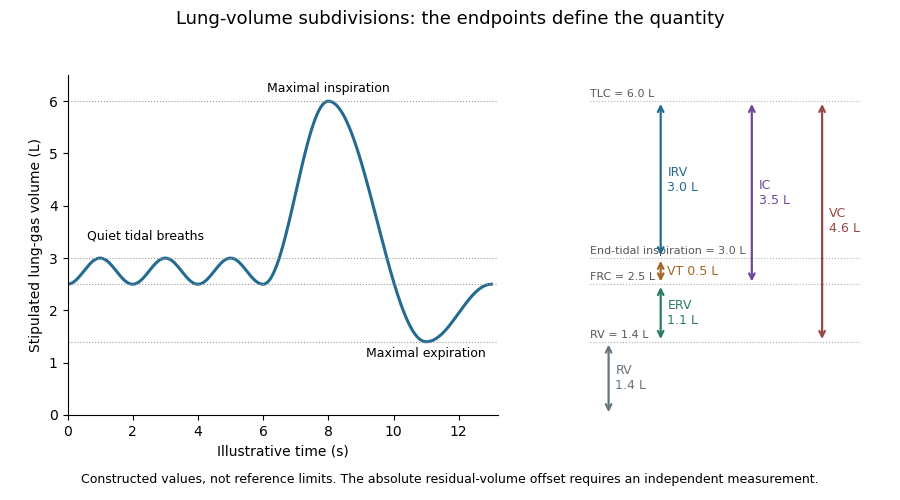
Vital capacity, VC, is the volume change between maximal inspiration and maximal expiration. It is the exchangeable difference between total lung capacity and residual lung volume:The sum uses inspiratory reserve volume, tidal volume and expiratory reserve volume.^[ref]

A constructed volume record with maximum 6.0 L and minimum 1.4 L gives VC 4.6 L. Subdivisions 3.0 L, 0.5 L and 1.1 L give the same result. Those increments partition the full excursion; none includes the 1.4 L that remains after maximal expiration.

Forced vital capacity names a specific forceful expiratory maneuver. The broader vital capacity can also be measured during a relaxed expiration or inspiration. The maneuver and completeness of its endpoints matter when comparing measurements.^[ref][ref]

A spirometry trace records volume change, so the same VC can arise at different absolute lung-gas levels. A second stipulated record spanning 7.0 to 2.4 L also gives 4.6 L. Adding a common offset to every point leaves VC unchanged. This is why a precise vital capacity measurement alone cannot determine residual lung volume or total lung capacity.

The distinction is useful experimentally: a large recorded excursion establishes how much gas was exchanged in that maneuver, while an independent absolute-volume measurement establishes how much gas occupied the lungs at its endpoints.

Inspiratory capacity, IC, is the maximum volume that can be inhaled from the end of a quiet expiration to maximal inspiration. Its lower reference is functional residual capacity, and its upper reference is total lung capacity:The last expression combines tidal volume with inspiratory reserve volume.^[ref]

For stipulated total lung capacity 6.0 L and functional residual capacity 2.5 L, IC is 3.5 L. If tidal volume is 0.5 L, the corresponding inspiratory reserve volume is 3.0 L. The two descriptions use the same maximum inspiratory endpoint but different starting points.

The starting point is essential when interpreting a change. In an original comparison, keep total lung capacity at 6.0 L while moving the quiet end-expiratory level from 2.5 to 3.2 L. IC falls from 3.5 to 2.8 L, although the maximum inspiratory volume has not changed. Thus a lower inspiratory capacity need not imply a lower total lung capacity; an independently specified baseline is required to distinguish the possibilities.

Inhalation through a volume-measuring apparatus can determine an inspiratory increment without directly measuring the gas already present in the lungs. A stable starting level and complete endpoint connect that increment to the defined capacity. The technical standard therefore links capacity maneuvers with an identified FRC-level measurement.^[ref] The values in the example illustrate endpoint bookkeeping rather than reference limits for a particular person.

Body plethysmography uses pressure and volume changes in an enclosing chamber to measure respiratory mechanics and compressible thoracic gas volume. For lung-volume measurement, a brief closed-airway effort relates gas compression inside the lungs to the chamber signal. The gas volume belongs to the instant of occlusion; it is not automatically residual lung volume.^[ref]

In the original 1956 experiment, Arthur B. DuBois and colleagues used an airtight chamber of approximately 600 L, a mouthpiece shutter, capacitance pressure transducers and a cathode-ray oscillograph. One signal represented mouth pressure and the other chamber pressure, converted to volume change through instrument calibration.^[ref] An open communication between mouth and alveolar gas during the closed-airway effort is essential to interpreting the mouth signal.

For an ideal isothermal gas amount, Boyle's law givesWith stipulated effective absolute gas pressure $P=100$ kPa, compression $\Delta V=-0.006$ L and increase $\Delta P=0.2$ kPa, the exact expression gives 3.006 L. Neglecting the product of small changes gives the first-order result $V\simeq -P\Delta V/\Delta P=3.0$ L. Here $\Delta V$ is the inferred lung-gas change, not an unconverted box-pressure reading.

If the measurement starts at quiet end-expiration, the interpreted lung-volume reference is functional residual capacity; linked inspiratory capacity and vital capacity maneuvers then provide other capacities. The thermal behavior of gas, instrument response and mouth-to-alveolar pressure equilibration remain physical assumptions to assess. A precise algebraic fit cannot repair a pressure signal that represents a different compartment.

Unlike tracer dilution, compression can probe gas that is not freely reached by the tracer during the test. This explains why body plethysmography and nitrogen washout can give different results without being duplicate names for the same observable.^[ref]

Nitrogen washout is a lung-gas measurement method that follows removal of resident nitrogen while the inspired gas contains little or no nitrogen. Gas analysis and expired volume are combined over multiple breaths to estimate the communicating gas volume.^[ref] It differs from adding helium and waiting for equilibration in helium dilution measurement of lung volume.

A conservation argument supplies the basic calculation. In an ideal compartment with unchanged gas volume $V$, initial and final nitrogen fractions $f_0$ and $f_T$, and net nitrogen volume $W$ removed,For stipulated $W=2.10$ L, $f_0=0.78$ and $f_T=0.01$, $V\simeq 2.73$ L. This is a simplified bookkeeping model with gas volumes compared at consistent conditions. Real equipment space and physiological gas exchange need their defined treatment.

The removed tracer is a volume-weighted quantity. For a nitrogen fraction $f(t)$ and positive expiratory volumetric flow rate $Q(t)$, an interval contributes $\int f(t)Q(t)dt$, with any inspired tracer subtracted for net removal. Two constructed expired parcels of 1 L at fraction 0.4 and 3 L at fraction 0.1 contain 0.7 L nitrogen in total. Multiplying their unweighted mean fraction 0.25 by total volume 4 L would instead give 1.0 L. Correct synchronization of gas and flow signals is therefore fundamental.

A long tail need not imply one uniformly slow compartment. In an original two-compartment model,the late signal is increasingly dominated by the slow component even if its initial amount $b$ was small. A finite stopping interval can consequently miss slowly communicating material. The washout curve, its integral and the functional residual capacity estimate describe different aspects of the same transport measurement.

Helium dilution measurement of lung volume estimates communicating lung-gas volume by mixing it with a known apparatus volume containing helium. The gas concentration changes as the tracer distributes through the connected space. Connection at the quiet end-expiratory level makes the result an estimate associated with functional residual capacity.^[ref]

In an ideal closed system with equal pressure and temperature, let $V_a$ be the known apparatus volume and $c_1$ its initial helium fraction. If the lung initially contains negligible helium and equilibration gives fraction $c_2$, conservation givesStipulated $V_a=2.4$ L, $c_1=0.10$ and $c_2=0.04$ give $V_L=3.6$ L. If that unknown space includes 0.2 L of external mouthpiece volume, the represented lung volume is 3.4 L. Instrument space and lung space must therefore be distinguished before naming the reported volume.

Equilibration also matters quantitatively. Stopping at an apparent fraction 0.05 instead of the modeled final 0.04 would give 2.4 L, an underestimate of 1.2 L in the uncorrected model. The sensitivity isAt the stated values, a small positive fraction error 0.001 changes the estimate by approximately $-0.15$ L. Correct concentration measurement and the stopping definition are thus parts of the volume measurement.

The technical apparatus includes a mixing circuit, helium analysis, carbon dioxide absorption and replacement of consumed oxygen.^[ref] These features keep other gas changes from masquerading as tracer dilution. Leaks, incomplete mixing and gas not communicating with the circuit violate different assumptions. Body plethysmography asks a complementary question about compressible thoracic gas volume; the two methods need not sample identical gas compartments.

Mechanical ventilation assists or replaces the movement of gas into and out of the lungs using a machine. A ventilator can deliver that assistance through a mask or a breathing tube.^[ref] This supports pulmonary ventilation; it does not replace every function of the lungs, circulation or gas exchange.

In positive-pressure ventilation, pressure applied at the airway opening helps drive inhalation. The resulting tidal volume depends on both that pressure history and respiratory mechanics. For a passive single-compartment model, a useful equation isHere $V$ is volume above the selected end-expiratory reference, $C$ is respiratory-system compliance, $R$ is airway resistance, and $p_0$ represents the baseline positive end-expiratory pressure. The model neglects active respiratory muscle pressure and changes in these coefficients.

For constructed $C=0.05$ L/cm H${}_2$O, $R=5$ cm H${}_2$O·s/L, $V=0.5$ L, $\dot{V}=0.5$ L/s and $p_0=5$ cm H${}_2$O, the predicted airway pressure is $5+10+2.5=17.5$ cm H${}_2$O. At zero flow with the same volume, the resistive term vanishes and the model gives 15 cm H${}_2$O. Thus an airway-pressure peak contains different information from a no-flow pressure measurement. These numbers illustrate the equation, not patient settings.

The importance of testing ventilation strategies was demonstrated by a 2000 randomized trial in acute respiratory distress syndrome and acute lung injury. It compared lower and traditional tidal volume strategies indexed to predicted body weight, with different plateau-pressure limits. In 861 participants, reported mortality was 31.0% versus 39.8%.^[ref] The experiment compared complete specified protocols in a defined population; it does not establish one universal setting from tidal volume alone. Physical models explain how pressure and flow interact, while controlled clinical evidence tests consequences that those models cannot supply by themselves.

Minute ventilation, ${\dot{V}}_E$, is the total volume of respiratory gas moved per unit time, conventionally expressed in litres per minute. When breath volumes are represented by mean tidal volume ${\overline{V}}_T$ and respiratory rate $f$ over the same interval,It measures gross ventilation, distinct from the portion renewing gas in effectively exchanging alveolar regions.^[ref]

An original record contains three complete expirations of 0.4, 0.6 and 0.5 L over 15 s. Their total is 1.5 L, giving $1.5\times 60/15=6$ L/min. The rate is 12 breaths/min and the mean tidal volume is 0.5 L, producing the same answer. Variable breath depth is therefore compatible with this identity if both summaries use the same record.

With a fixed effective respiratory dead space $V_D$ per breath, the corresponding model for alveolar ventilation isFor the constructed record and $V_D=0.15$ L, the effective volume is $1.5-3(0.15)=1.05$ L per 15 s, or 4.2 L/min. The remaining 1.8 L/min belongs to the modeled dead-space turnover. This subtraction assumes each included breath exceeds the modeled dead-space volume.

A pneumotachograph can supply signed volumetric flow rate for integration. Integrating only the expiratory phase yields expired volume; integrating a full balanced breath with its sign intact yields approximately zero net volume. A ventilation report must consequently identify the phase, interval and gas-volume conditions rather than interpreting every integral as the same quantity. Gross minute ventilation alone does not establish oxygen uptake, carbon-dioxide removal or their distribution among lung regions.

Respiratory dead space describes ventilated gas volume that does not contribute to the gas exchange represented by the chosen measurement. Anatomical dead space concerns conducting airways; alveolar dead space concerns ventilation of alveolar regions with ineffective exchange relative to their perfusion. The definition and estimator must be stated before the number is interpreted.^[ref]

A two-compartment carbon dioxide balance illustrates the gas-exchange estimate. Suppose inspired gas contains negligible carbon dioxide, a dead-space fraction contributes none, and the remaining expired volume carries representative alveolar fraction $F_A$. For mixed expired fraction $F_E$,Stipulated $F_A=0.05$ and $F_E=0.035$ give a dead-space fraction 0.30. With tidal volume 0.50 L, the corresponding effective dead-space volume is 0.15 L. This is a dilution-model result, not proof that a conducting tube of exactly that physical volume exists.

The alveolar quantity in the equation is important. Replacing it with an arterial carbon-dioxide measurement adds physiological assumptions and can reflect more than conducting-airway volume. The technical account distinguishes the alveolar balance from its arterial substitution.^[ref]

An original comparison makes the distinction concrete. Two modeled systems each have anatomical dead space 0.15 L. In one, all remaining inspired gas reaches effectively exchanging regions. In the other, an additional 0.10 L per breath goes to a ventilated region that does not exchange with perfusing blood. Their effective dead-space volumes are 0.15 and 0.25 L despite the same conducting geometry.

The label therefore belongs to a specified physical or physiological model. A measured dead-space fraction, a geometrical airway volume and an estimate of wasted ventilation are related observations, rather than automatically interchangeable measurements.