For a nonidentity Möbius transformation whose two fixed points are antipodal under stereographic projection, conjugate by a sphere rotation sending them to $0,\infty$. The conjugated map fixes both, hence is $z\mapsto az$ with $a\ne 0$. If $|a|=1$ it is an axial rotation; if $|a|<1$ every finite orbit tends to zero; if $|a|>1$ every nonzero orbit tends to infinity. Undoing the rotation gives either a sphere rotation or one attracting fixed point with the other as the sole exceptional initial point.

Let $T_a(z)=z+a$, $S_k(z)=kz$ with $k\ne 0$, and $I(z)=1/z$ on the Riemann sphere. For $F(z)=(az+b)/(cz+d)$ and $\Delta =ad-bc\ne 0$, $c=0$ gives $F=T_{b/d}\circ S_{a/d}$. If $c\ne 0$, division gives $F=T_{a/c}\circ S_{-\Delta /c^2}\circ I\circ T_{d/c}$. The expressions agree at poles and at infinity by the sphere conventions. These elementary maps therefore generate the Möbius transformation group.

The Möbius transformations generated by $D_{\lambda }(z)=\lambda z$ with $\lambda \ne 0$ and $I(z)=1/z$ have exactly the two displayed forms. The relations $I^2=1$ and $I{D}_{\lambda }=D_{{\lambda }^{-1}}I$ reduce every word to $D_{\lambda }{I}^{ϵ}$, $ϵ\in \{0,1\}$. This is a semidirect product of ${\mathbb{C}}^{\times }$ with a cyclic group of order two acting by multiplicative inversion. It preserves the unordered pair $\{0,\infty \}$, and only its scaling elements fix zero.

The Möbius transformations preserving a three-point set act faithfully on it: one fixing all three is the identity. Every permutation is realized because a Möbius transformation can send any ordered distinct triple to any other, by composing the two normalizations to $0,1,\infty$. For that normalized set the six maps are $z$, $1-z$, $1/z$, $1/(1-z)$, $z/(z-1)$ and $(z-1)/z$. Thus its setwise stabilizer is the symmetric group $S_3$. Normalizing any other three-point set conjugates its stabilizer to this group.

For two distinct points of the Riemann sphere, conjugate by a Möbius transformation sending them to zero and infinity. A transformation fixing those two points has the form $z\mapsto \lambda z$, $\lambda \ne 0$. Composition multiplies the parameter, so the pointwise stabilizer is isomorphic to the complex multiplicative group. For zero and one, conjugation by $z/(1-z)$ gives $z\mapsto \lambda z/[1+(\lambda -1)z]$.

In the quotient space description of the Möbius band, follow $v=+1$ once along the rectangle. The seam sends its endpoint to the start of $v=-1$, which must also be traversed before returning to the original point. Under the deformation retraction onto the core circle of a Möbius band, these two stretches each travel once around the same circle. Orienting both circles by increasing longitudinal parameter gives a map of topological degree two. Equivalently, the group homomorphism on fundamental groups induced by inclusion of the boundary sends a chosen generator to twice the core generator, or to $c^2$ in multiplicative notation. Reversing the chosen boundary generator changes the sign, not the fact that it winds twice.

For the model $F$ of the Möbius band, the tangent vectors along its core circle of a Möbius band areTheir cross product, divided by its norm $R$, gives the continuous unit normalAlthough $F(2\pi ,0)=F(0,0)$, we have $n(2\pi )=-n(0)$. Any other continuous choice of unit normal along this parametrized interval is either $n$ everywhere or $-n$ everywhere: its relative sign is a continuous map into the discrete space $\{+1,-1\}$, and the interval is connected. Thus no choice can agree at the identified endpoints. This short calculation proves that the Möbius band has no global continuous unit normal and is not an orientable surface.

The plotted quantity is $n(\theta )\cdot n(0)=\cos (\theta /2)$. It compares ambient vectors at generally different points; after one circuit it is $-1$ at the starting point, and after two circuits it is $+1$ there. Only these endpoint comparisons are needed for the orientability argument.

The core circle is the image of the centre line in the rectangle defining a Möbius band. Its endpoints are identified, so it is a circle. The formuladefines a deformation retraction onto that circle: it respects $(0,v)\sim (1,-v)$, starts at the identity map, and fixes the core throughout. Consequently the Möbius band has fundamental group isomorphic to $\mathbb{Z}$, just like a circle; this alone cannot distinguish it from an annulus.

For a two-component mixture model with known component tail probabilities $p_0,p_1$ above a threshold, the overall probability is $p(q)=(1-q)p_0+q{p}_1$. An empirical exceedance fraction $\hat{p}$ gives the displayed method-of-moments estimate when $p_1\ne p_0$. Under independent observations, the exceedance count has a binomial distribution, and its constrained maximum-likelihood estimate is the same expression clipped to $[0,1]$. Equal component tail probabilities make this summary uninformative about $q$.

The displayed mixture distribution combines a Standard Cauchy distribution and a symmetric law whose magnitude has cumulative distribution function $r^2/(1+r^2)$ for $r\ge 0$. Use independent uniforms $U,V,H$: if $U\le p$, return $\tan (\pi (V-1/2))$; otherwise return a fair independent sign times $\sqrt{V/(1-V)}$. The magnitude density is $2r/(1+r^2{)}^2$ and splitting its mass equally between signs gives $|x|/(1+x^2{)}^2$. An alternative rejection sampling proposal is standard Cauchy, with envelope constant $M=p+\pi (1-p)/2$, because $|x|/(1+x^2)\le 1/2$.

A Gaussian mixture distribution is a weighted sum of normal distribution densities, with nonnegative weights summing to one. It need not itself be a normal distribution: components with different means and variances can produce skewness or several modes. Its raw moments are weighted sums of the component moments.

Prepare the auxiliary register in the maximally mixed state $I/N$ and estimate both mixed-state Hadamard-test quadratures. Multiplying the normalized expectation by $N$ estimates the trace of $U$. A uniformly randomized preparation of any orthonormal basis produces $I/N$; the eigenvectors of $U$ need not be known.

For fixed $0<p<1$, the missing common-neighbour count in a binomial random graph has expectation tending to zero. The Markov inequality therefore shows that every pair has a common neighbour with probability tending to one. On that event every graph distance is at most two, so the graph is connected and its graph diameter is at most two.

For ${\alpha }^3=6$, the ring of integers is $\mathbb{Z}[\alpha ]$ and its field discriminant is $-972$. The Minkowski bound for ideal classes is $16\sqrt{3}/\pi <9$. Prime ideals of norm at most eight lie above $2,3,5,7$. The primes above two, three and the degree-one prime above five are generated by $\alpha -2$, $3+2\alpha +{\alpha }^2$ and $\alpha -1$, of norm magnitudes $2,3,5$. At seven the residue roots are $3,5,6$; the primes at roots six and three are generated by $\alpha +1$ and ${\alpha }^2+\alpha -5$, both of norm seven. Their product with the remaining prime is $(7)$, making that prime principal too. Every possible Minkowski representative is therefore principal.

Distinct spacetime events have null separation when their displacement has zero Minkowski interval, equivalently $c|\Delta t|=|\Delta \mathbf{x}|$. They can be joined by a straight vacuum light ray. Their nonzero displacement is a null vector, so the zero squared interval does not mean that the spacetime events coincide. For example, $(t,x)=(3\mathrm{s},3\mathrm{ls})$ is null separated from the origin.

Two distinct spacetime events have timelike separation when their displacement has negative Minkowski interval in metric signature $(-,+,+,+)$, equivalently $c|\Delta t|>|\Delta \mathbf{x}|$. A massive observer can connect them along a straight timelike curve. If the later spacetime event has $\Delta t>0$, every Lorentz transformation in the orthochronous Lorentz group keeps it later. The elapsed proper time on the straight inertial segment is $\sqrt{-s^2}/c$.

In the light-second units of the Minkowski spacetime example, $O$ to $A$ has $s^2=(-4^2+3^2){\mathrm{ls}}^2=-7{\mathrm{ls}}^2$. Its straight moving clock therefore records $\sqrt{7}\mathrm{s}$, approximately $2.646\mathrm{s}$, while the coordinate time difference is $4\mathrm{s}$. Coordinate time and proper time answer different questions.

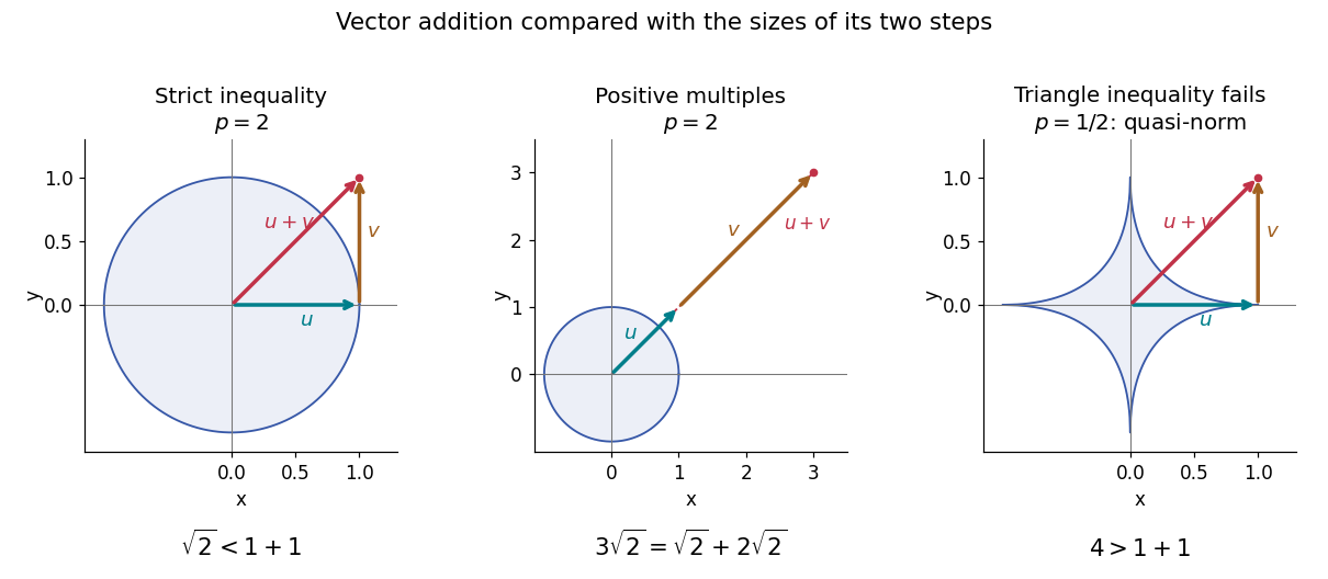
For $0<p<1$, write $Q_p(f)=(\int |f{|}^{p}d\mu {)}^{1/p}$ to emphasize that this is a quasi-norm, as in the Lq quasi-norm branch. On two coordinates with counting measure, $u=(1,0)$ and $v=(0,1)$ give $Q_p(u)=Q_p(v)=1$, but $Q_p(u+v)=2^{1/p}>2$. At $p=1/2$, this is the explicit failure $4>1+1$ in the right panel of the diagram. The midpoint $(1/2,1/2)$ has $Q_p=2^{1/p-1}>1$, so the corresponding unit sublevel set is not a convex set.

A useful replacement survives: for nonnegative real numbers $a,b$, $(a+b{)}^p\le a^p+b^p$. Together with the scalar triangle inequality, this yieldsConsequently $d_p(f,g)=Q_p(f-g{)}^p$ is a metric on the equivalence classes of measurable functions with finite $Q_p$, even though $Q_p(f-g)$ itself need not be a metric. Do not replace the failed Minkowski inequality by a universal reversed bound for signed or complex functions: $g=-f\ne 0$ would give a zero sum but two positive separate sizes.

Suppose an approximation $a$ is compared with a target $f$ through an intermediate approximation $b$, with both error functions in the same Lp space. The identity $f-a=(f-b)+(b-a)$ and the Minkowski inequality combine two error budgets without any independence assumption. The L1 norm controls aggregate absolute error, the L2 norm controls the square root of aggregate quadratic loss, and the L-infinity norm controls the largest error almost everywhere. For equally weighted samples with the probability measure $1/n$ on each coordinate, the L2 norm is the root mean square error; the inequality still applies when this normalization is used consistently.

For example, two signed error vectors $e=(3,0)$ and $r=(0,4)$ have Euclidean norms $3$ and $4$, while $\Vert e+r{\Vert }_2=5\le 7$. Reinforcing errors $e=(3,0)$ and $r=(4,0)$ attain the bound $7$; opposing errors $e=(3,0)$ and $r=(-3,0)$ cancel completely. The Minkowski inequality always allows reinforcement. A smaller combined budget requires additional information about the errors, not just their separate norms.

Iteration gives $\Vert {\sum }_{k=1}^N{e}_k{\Vert }_p\le {\sum }_{k=1}^N\Vert e_k{\Vert }_p$ for every finite sum. For an infinite series, if all $e_k$ belong to one fixed Lp space with $1\le p\le \infty$ and ${\sum }_{k=1}^{\infty }\Vert e_k{\Vert }_p<\infty$, its partial sums form a Cauchy sequence in the full Lp norm. Completeness of this Banach space then gives norm convergence to an element of the same Lp space. A finite sum bound alone does not establish convergence, and completeness is an additional ingredient beyond the Minkowski inequality. ^[ref]

For $1<p<\infty$ and nonzero elements $f,g$ of the same real or complex Lp space, equality in the Minkowski inequality holds if and only ifEquivalently, $g=cf$ almost everywhere for a single positive real number $c$. The multiplier must be constant across $X$; matching signs at each input alone is insufficient. For complex numbers, an arbitrary complex scalar multiple is also insufficient: $g=if$ gives $\Vert f+g{\Vert }_p=\sqrt{2}\Vert f{\Vert }_p<2\Vert f{\Vert }_p$ for nonzero $f$. If either element is zero in Lp space, equality holds automatically, even if a representative has nonzero values on a null set.

The reason is strictly convex normed space geometry. Normalize $f,g$ to unit Lp norm and use weights $\Vert f{\Vert }_p/(\Vert f{\Vert }_p+\Vert g{\Vert }_p)$ and $\Vert g{\Vert }_p/(\Vert f{\Vert }_p+\Vert g{\Vert }_p)$. Distinct normalized functions give a convex combination of Lp norm strictly below one. This follows by integrating the strict convexity of $z\mapsto |z{|}^p$ on the real numbers or complex numbers; equality therefore forces the normalized functions to agree almost everywhere.

At $p=1$, equality instead means $|f+g|=|f|+|g|$ almost everywhere: the nonnegative difference has zero integral. For real functions, this is $fg\ge 0$ almost everywhere. For complex functions, their nonzero values must have the same argument wherever both are nonzero, but their magnitude ratio may vary. The disjoint-coordinate vectors $(1,0)$ and $(0,1)$ illustrate equality without constant proportionality.

At $p=\infty$, no such constant proportionality condition is necessary: $(1,0)$ and $(1,1)$ have L-infinity norms one and a sum of L-infinity norm two. Nor must an essential supremum be attained: under Lebesgue measure on $(0,1)$, $f(x)=g(x)=x$ give equality $2=1+1$, although neither function takes the value one. The endpoint Lp spaces need not be strictly convex normed spaces.

For vectors $u,v\in {\mathbb{R}}^n$ or ${\mathbb{C}}^n$, counting measure turns the Minkowski inequality intoFor $p=\infty$, replace each displayed norm by the maximum of its coordinate absolute values. Take $u=(1,0)$ and $v=(0,1)$. Both vectors have Lp norm one for every $p\ge 1$, but their sum has L1 norm $2$, Euclidean norm $\sqrt{2}$, and L-infinity norm $1$. Thus the same vector addition gives equality $2=1+1$ at $p=1$, strict inequality $\sqrt{2}<1+1$ at $p=2$, and strict inequality $1<1+1$ at $p=\infty$.

By contrast, $u=(1,1)$ and $v=2u=(2,2)$ give equality for every $p\ge 1$: absolute homogeneity of a norm yields $\Vert u+v{\Vert }_p=3\Vert u{\Vert }_p=\Vert u{\Vert }_p+\Vert v{\Vert }_p$. At $p=2$, the three sizes are $\sqrt{2}$, $2\sqrt{2}$, and $3\sqrt{2}$. Opposite vectors behave very differently: $u+(-u)=0$, so the inequality is strict whenever $u$ is nonzero. Cancellation is allowed; the bound describes the largest possible total size.