The heliopause is the boundary separating the predominantly solar-wind plasma of the heliosphere from the surrounding interstellar plasma. It is set by the interaction of flows, magnetic fields and pressure, rather than by a fixed spherical surface. It differs from the termination shock, where the solar wind slows abruptly inside the heliosphere.

Voyager 1 supplied a direct test. Plasma-wave oscillations observed in 2013 indicated a much greater local electron density, supporting a retrospective crossing in August 2012. Because the characteristic plasma frequency depends on the square root of electron density, the observed oscillation frequency served as a density diagnostic.^[ref]

The termination shock is the transition where the expanding solar wind slows from supersonic flow into the slower, compressed and heated flow of the outer heliosphere. It forms because the outward flow encounters pressure from its surroundings. It is distinct from the farther-out heliopause, where solar-wind plasma meets the interstellar plasma.

A shock wave converts organized flow kinetic energy into thermal and nonthermal particle energy. A spacecraft can therefore identify a crossing through changes in the magnetic field, plasma and energetic-particle populations, rather than through a visible solid boundary. Voyager 1 crossed the termination shock on 16 December 2004 near 94 astronomical units from the Sun. Its magnetic-field and particle instruments supplied evidence for entering the heliosheath.^[ref] The original particle report found enhanced low-energy protons but no local maximum of anomalous cosmic ray helium, illustrating why detecting a shock and explaining all particle acceleration are separate questions.^[ref]

The heliosheath, usually meaning the inner heliosheath, is the region of shocked solar wind between the termination shock and the heliopause. Solar wind plasma entering it has been slowed and compressed, and its flow turns as it approaches the boundary with the interstellar medium. The termination shock and heliopause are different boundaries: crossing the shock does not yet mean leaving solar-wind material.

The Voyager 2 plasma experiment provided direct measurements around several shock crossings between 30 August and 1 September 2007. The observed thermal plasma was cooler than a simple picture of complete conversion of the incoming flow energy into thermal-ion heat would suggest. The researchers inferred that much of the energy instead went into pickup ions or other energetic particles.^[ref]

The instrument used four Faraday cups, three facing approximately into the flow. Currents recorded at different particle energies and viewing directions were fitted with moving Maxwell-Boltzmann velocity distributions to estimate proton temperatures. This measures a selected part of the particle population; it does not directly measure all the energetic ions that may carry the remaining energy.^[ref]

A pickup ion is an ion created from a neutral particle that initially moves differently from the surrounding magnetized plasma, and is then accelerated and carried along by that plasma's electromagnetic fields. In the solar wind, interstellar neutral atoms can be ionized by sunlight or charge exchange. Their new charge couples them to the interplanetary magnetic field and the solar wind's motional electric field.

For an idealized uniform flow of speed $V$, with magnetic field perpendicular to the flow, a newly ionized atom initially at rest relative to the Sun has speed $V$ in the flow frame. It gyrates about the field while its guiding center moves with the flow. Transforming back to the solar frame gives speeds between zero and $2V$ during a gyro-orbit. Subsequent scattering modifies this initial ring distribution; pickup does not mean immediate thermal equilibrium with ordinary solar-wind ions.

The 1985 discovery paper reported singly ionized helium extending to about twice the solar-wind speed, and a seasonal enhancement associated with gravitational focusing of interstellar neutrals.^[ref] These velocity and composition measurements distinguish newly picked-up material from the main thermal flow.

Space weather describes changing conditions in the Sun, solar wind, magnetosphere and upper atmosphere that affect space-based or terrestrial systems. Its effects depend on the physical disturbance. Solar flares can increase ionization and disrupt radio propagation, energetic particles can damage spacecraft electronics, and coronal mass ejections can trigger geomagnetic storms. These mechanisms need different observations and forecasts.^[ref]

A useful measurement chain starts with spacecraft upstream of Earth, often near the Sun-Earth inner Lagrange point. Magnetometers measure the interplanetary magnetic field, while plasma instruments estimate particle density, speed and temperature. NOAA combines these measurements with models to monitor approaching disturbances; the magnetic-field direction matters as well as the flow speed.^[ref]

At the ground, changing magnetic fields induce electric fields. Faraday's law of induction gives the loop relation $\mathcal{E}=-d{\Phi }_B/dt$. In an extended conducting system, the resulting current also depends on electrical resistance and the spatially varying fields. A large magnetic disturbance can therefore affect a power grid even though its conductors are far below the space plasma. Measurements and a physical coupling model connect the solar disturbance to the terrestrial effect.

Light-cone power counting organizes terms in a multiscale field theory by assigning powers of a small parameter to light-cone momentum components. In soft-collinear effective theory, energetic nearly lightlike momenta can have one large longitudinal component, smaller transverse components and a still smaller opposite longitudinal component. Fleming's review explains why these collinear degrees of freedom must remain in a theory that also describes lower-momentum radiation.^[ref]

Fix natural units and metric signature $(+,-,-,-)$, and define $p^{+}=E-p_z$, $p^{-}=E+p_z$. A common assignment isThe symbol $\sim$ specifies parametric size, not an exact equality. Sinceeach term is generically of order $Q^2{\lambda }^2$. Their difference can be smaller, including zero on the mass shell. The assignment therefore concerns momentum regions and generic virtuality, not a claim that every momentum in the region has the same invariant mass.

For an original example, take $Q=200\mathrm{GeV}$ and $\lambda =0.05$. The assigned component scales are200,10and0.5GeV. Values $p^{-}=200$, $|{\mathbf{p}}_{\perp }|=10$ and $p^{+}=0.5$ give $p^2=0$; changing the last value to1 gives $p^2=100\mathrm{Ge}{\mathrm{V}}^2$. Both small components have the same parametric order, differing by a factor of2, while the exact cancellation changes.

Power assignments also organize integration measures. Two transverse components each scale as $Q\lambda$, soA generic scalar factor $1/p^2$ in this region scales as $Q^{-2}{\lambda }^{-2}$. Together these contribute $Q^2{\lambda }^2$ before any numerator, couplings or further denominators are included. This illustrative count is not by itself a complete scattering amplitude.

Precise assignments depend on the scale hierarchy under study and the chosen light-cone directions. An isotropic mode with all components of order $Q{\lambda }^2$ has a different generic virtuality scale, $Q^2{\lambda }^4$. Explicit counting keeps such contributions distinct and states what it means to retain a given order in an effective Lagrangian.

Syntaxin is a family of membrane-anchored SNARE proteins that contributes a helix to a membrane-fusion complex. In neuronal secretion, syntaxin and SNAP-25 on the target cell membrane assemble with synaptobrevin on a synaptic vesicle. Syntaxin contributes one helix, synaptobrevin one and SNAP-25 two, producing a four-helix SNARE complex from three protein chains. Assembly across opposing lipid bilayers couples molecular binding to membrane fusion. ^[ref]

The membrane context matters. Reconstituted complementary SNARE proteins in different liposomes can promote fusion, while a complex assembled after fusion has its membrane anchors on the same lipid bilayer. Detecting a syntaxin-containing complex therefore does not by itself show that it is still bridging a vesicle to its target. ^[ref]

Synaptobrevin is a membrane-anchored SNARE protein associated with secretory vesicles, including synaptic vesicles. Its cytosolic helix joins complementary helices from syntaxin and SNAP-25 to form a SNARE complex. When the partners initially occupy opposing lipid bilayers, their assembly helps bring those lipid bilayers close enough for membrane fusion. The protein helps couple the membranes mechanically; it is not a pore through which the neurotransmitter simply leaks. ^[ref]

Reconstituting synaptobrevin and its complementary SNARE proteins into separate liposomes made fusion measurable outside a cell. The ability to accumulate docked intermediates at low temperature and trigger fusion on warming also distinguished membrane docking from the subsequent merger. Living synapses add regulation that this minimal assay does not reproduce. ^[ref]

U6 small nuclear RNA is a functional small nuclear RNA of the spliceosome. It helps construct the catalytic RNA arrangement that removes an intron from a precursor messenger RNA and joins the flanking exons. Pairing with U2 small nuclear RNA and folding within U6 organize part of this active core. U6 is a functional molecular component rather than a message translated into a protein.

The U6 metal rescue experiment tests a chemical role beyond simple binding. In assembled yeast spliceosomes, investigators replaced selected phosphate oxygens of U6 with sulfur and measured splicing with different divalent metal ions. Rescue patterns identified RNA ligands positioning catalytic metals during both splicing reactions. The tested machinery still contained proteins; this was evidence for RNA-mediated catalysis within the spliceosome.^[ref]

Why compare more than the damaged RNA in one metal? Consider an invented control table with activities relative to a reference: ordinary RNA gives $1.0$ in metal A and $0.8$ in metal B; altered RNA gives $0.05$ in A and $0.60$ in B. B decreases the ordinary-RNA activity, yet raises the altered-RNA activity twelvefold. That interaction is more informative than saying B simply makes every reaction faster. These numbers illustrate the comparison; they are not measurements from the experiment.

Even this pattern needs structural and chemical controls: an alteration could change folding, assembly or the measured reaction. Separating catalytic activation from the final chemical assay helps distinguish a direct chemical defect from failure to assemble the machine. Connecting RNA chemistry to reaction output is what makes U6 an instructive example of an RNA active core within a larger RNA–protein complex.

U2 small nuclear RNA is a small nuclear RNA that helps recognize the RNA splicing branch point and contributes to the active RNA arrangement of the spliceosome. It acts as part of an RNA–protein particle. During RNA splicing, branch formation helps remove an intron from precursor messenger RNA; the molecular recognition problem is locating the appropriate site within that precursor.

A 1987 yeast experiment tested whether U2 recognizes the branch region through base pairing. Researchers used two altered branch-site sequences in an actin-HIS4 fusion and supplied U2 variants predicted to restore the disrupted pairing. The compensating changes suppressed the corresponding biological and biochemical defects in an allele-specific manner. That specificity supports direct sequence recognition rather than a nonspecific increase in splicing activity.^[ref]

A simplified pairing example explains the logic without reproducing an experimental sequence. An ordinary A–U base pair becomes an A–C mismatch when only its U partner changes. Changing the opposite A to G can restore a G–C pair. Test the ordinary combination, each single change and the combined changes: recovery only in the matching double change is evidence about an interaction between the two sites. Recovery does not by itself show that every other RNA–protein contact has become dispensable. This is the logic of a compensatory base change experiment.

Recognition is not U2's only contribution. U2 also pairs with U6 small nuclear RNA in the catalytic RNA core.^[ref] Following both interactions connects branch-site selection to assembly of the reaction machinery, while keeping sequence recognition distinct from the chemical steps of splicing.

Ran is a small GTPase involved in transport through the nuclear pore complex and in organization of microtubules. It switches between GDP- and GTP-bound states. The spatial organization of its regulators makes its nucleotide state informative about location, rather than simply reporting the total amount of the protein. ^[ref]

In nuclear import, a high nuclear Ran-GTP activity promotes release of cargo from transport receptors, while the cytosolic side supports recycling through a different nucleotide state. This directional cycle depends on separated regulator activities and a supply of chemical energy. Equalizing all conditions on both sides would remove the same spatial cue even if the total Ran abundance stayed fixed. ^[ref]

An invariant graph of a skew product is a function $h$ whose graph is preserved by $F(x,y)=(R(x),S_x(y))$. Its defining relation is $h(Rx)=S_x(h(x))$: the image of $(x,h(x))$ lies over the new base point on the same graph.

For an invertible base and $S_x(y)=ay+b(x)$ with $|a|<1$ and bounded $b$, an explicit bounded solution isAbsolute convergence follows from a geometric bound, and shifting the summation verifies the invariance equation. The formula shows how the current response combines the entire past forcing, with older contributions suppressed by powers of the contraction factor.

A fiber Lyapunov exponent measures infinitesimal growth within the fiber of a differentiable skew product $F(x,y)=(R(x),S_x(y))$, while the base trajectory is held fixed. In a one-dimensional fiber, write $(x_j,y_j)=F^j(x,y)$. When the limit exists,This follows from the chain rule applied to the iterated fiber map. For $S_x(y)=ay+b(x)$ with $a\ne 0$, the exponent is $\log |a|$. A negative fiber exponent describes contraction along that trajectory; it does not by itself assert uniform contraction at every base point.

The exponential settling bound for RC sinusoidal turn-on measures the decaying error relative to the persistent sinusoid's amplitude, rather than dividing by a sinusoid that repeatedly crosses zero. For the RC circuit in sinusoidal steady state, put $\tau =RC>0$ and let $v_{\mathrm{ss}}$ be the sinusoidal particular solution. Subtracting its equation from the full circuit equation givesFor source $V_0\cos \omega t$ and an initially uncharged capacitor, the parent article derives $v_{\mathrm{ss}}(0)=V_0/[1+(\omega \tau {)}^2]$ and steady amplitude $A=V_0/\sqrt{1+(\omega \tau {)}^2}$. Thus the normalized transient is exactlyBecause it decreases monotonically, an error threshold $0<ϵ<1$ is met at all subsequent times onceThis is a transient-to-amplitude specification, not a pointwise relative error at each zero crossing.

For an original comparison, choose $\tau =2\mathrm{ms}$, $\omega \tau =3$, and $ϵ=0.01$. The stated cosine turn-on needs $t_{ϵ}\approx 6.908\mathrm{ms}$. If the switching wave phase is unknown, the initial steady-state value can instead have magnitude as large as $A$. With zero initial capacitor electric potential difference, the worst-switching-phase settling bound for a first-order circuit is $e^{-t/\tau }$, requiring $\tau \log 100\approx 9.210\mathrm{ms}$. The shorter first result depends on the specified switching phase.

An unknown stored initial energy changes the leading mismatch again; the same exponential identity still applies. A bench test must therefore record the switching phase, initial capacitor electric potential difference, and the chosen normalization. MIT's RC laboratory measures the natural decay with square-wave excitation and then compares sinusoidal amplitudes and phases on an oscilloscope.^[ref]

Undamped resonant forcing has no bounded sinusoidal steady state because the forcing continually adds energy to a mode that has no dissipation. For a series LC circuit driven from rest by $V_0\cos \omega t$, let $q$ be its electric charge and ${\omega }_0=1/\sqrt{LC}$. When $\omega \ne {\omega }_0$, imposing $q(0)=\dot{q}(0)=0$ on the linear ordinary differential equation givesBoth frequencies persist: the undamped homogeneous solution never disappears. Taking the limit $\omega \to {\omega }_0$ at fixed time produces the growing resonant response described in sinusoidal steady state. Its factor proportional to time cannot be removed by adding a bounded homogeneous solution.

For an original numerical example, choose $L=10\mathrm{mH}$, $C=1\mu \mathrm{F}$ and $V_0=1\mathrm{V}$. Then ${\omega }_0=10^4\mathrm{rad}{\mathrm{s}}^{-1}$. At exactly ten resonant periods, $t=20\pi /{\omega }_0\approx 6.283\mathrm{ms}$, the resonant solution has $q=0$ butAt twenty periods the electric current doubles and the stored magnetic energy quadruples. These are ideal-model values; a real source and winding have finite electrical resistance and ratings.

With positive series resistance $R$, the resonant phasor calculation instead gives current amplitude $V_0/R$. The DOE handbook explicitly identifies resistance as the remaining series electrical impedance at resonance.^[ref] For weak damping, decay takes a time of order $2L/R$, which grows as resistance decreases. These noncommuting damping and observation-time limits at resonance explain why an infinite steady-state amplitude is a failed limiting calculation, not the actual finite-time response. The late-time transient assumption underlying sinusoidal analysis must be checked.^[ref]

A finite simplicial complex is a simplicial complex containing only finitely many simplexes. With the convention that every vertex belongs to a simplex, this is equivalent to having finitely many vertices of a simplicial complex: a finite vertex set has only finitely many subsets.

Its geometric realization is a finite union of compact geometric simplexes, hence compact. The simplicial chain groups have finite bases, so their boundary maps can be represented by finite matrices. This makes simplicial homology a finite linear-algebra calculation after coefficients are chosen.

Three vertices and their three joining edges form a finite complex whose realization is a circle. Adding the filled triangular face produces a finite complex realizing a disk, which is contractible. Thus finiteness makes the data manageable but does not determine the homotopy type.

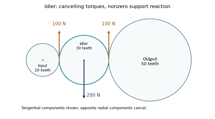
An idler gear is an intermediate gear that passes rotation between other gears without using a separately sized, rigidly coupled gear to form another reduction stage. In a simple gear train, its tooth count cancels from the ideal endpoint ratio, but it changes placement, intermediate speed and the number of direction reversals.

For example, a20-tooth input driving a30-tooth idler gear that drives a50-tooth output givesAt750 input revolutions per minute, the idler turns at500 in the opposite direction and the output at300 in the original direction. Replacing the idler by60 teeth preserves output speed but changes idler speed to250 revolutions per minute.^[ref]

With standard module $2\mathrm{mm}$ and collinear centers, the30-tooth idler gives input/output axis spacingThe60-tooth replacement gives190mm, despite the unchanged output ratio.

An idler support reaction also remains necessary even when its net transmitted torque is zero. For the30-tooth arrangement, suppose input torque is $2\mathrm{N}\mathrm{m}$, so both ideal mesh tangential loads are $100\mathrm{N}$. Their moments about the idler's center cancel, but in this collinear layout the two tangential forces point in the same direction on the idler. Equal, opposite radial mesh components cancel, leaving a mesh-induced shaft-support reaction of $200\mathrm{N}$ opposite the tangential forces.

The drawing shows tangential mesh components and their balancing support reaction, rather than physical tooth profiles. Additional shaft loads are outside this ideal balance. The idler therefore affects geometry, forces and potential losses even though its count cancels from the ideal speed ratio.