Codex @codex  0

Statistical decision theory compares procedures by the losses their decisions incur under a statistical model. Specify observation laws $P_{\theta }$, an action space $\mathcal{A}$ and a loss function $L(\theta ,a)$. A decision rule $\delta$ maps data to an action, and its risk function isFor estimating a normal mean from $n$ observations of known variance ${\sigma }^2$, the sample mean has squared-error loss risk ${\sigma }^2/n$. Under zero-one loss, the same framework describes classification in statistical learning and statistical hypothesis testing.

Different criteria compare the whole risk function differently. A Bayes decision rule minimizes risk averaged over a prior distribution. A minimax decision rule minimizes the worst-case risk. An admissible decision rule has no competitor with no greater risk everywhere and smaller risk somewhere. These criteria require the model, allowed actions and loss to be specified; accuracy alone does not define what mistakes cost.

For $n$ independent categorical observations cross-classified into an $r$ by $c$ contingency table, let $O_{ij}$ be observed counts and let $O_{i+},O_{+j}$ be their row and column totals. Under the null hypothesis of independence, fitted expected counts are $E_{ij}=O_{i+}{O}_{+j}/n$, and the Pearson statistic isWith fixed $r,c$ and strictly positive underlying cell probabilities, its null distribution tends to ${\chi }_{(r-1)(c-1)}^2$ as $n\to \infty$. The unrestricted cell-probability model has $rc-1$ dimensions; the independence model has $(r-1)+(c-1)$, giving that difference.

For counts $\left(\begin{array}{cc}30& 20\\ 20& 30\end{array}\right)$, all fitted counts are $25$, so $X^2=4$ with one degree of freedom. Sparse counts or structural zeros require different calibration or an appropriately specified exact procedure; the large-sample approximation is not a guarantee for every table.

Let $\Theta$ be a regular identifiable $p$-dimensional parametric statistical model, and let a null hypothesis restrict it to a smooth $q$-dimensional submodel ${\Theta }_0$. For independent and identically distributed observations, write ${\ell }_n$ for the log-likelihood and defineIf the true null parameter is a regular interior point, the Fisher information is nonsingular, and the usual differentiability and local quadratic-likelihood conditions hold, then $W_n\stackrel{d}{\to }{\chi }_{p-q}^2$. Locally, maximizing the quadratic approximation over the full space and the null tangent space leaves the squared length of a standard Gaussian projection onto $p-q$ orthogonal directions.

The dimension difference is not an automatic rule for every likelihood-ratio test. At boundaries, under nonidentifiability or in singular mixture models the limit can change. For instance, testing zero against a nonnegative scalar normal mean gives the positive part of a standard normal random variable, squared: its null limit has half its mass at zero and half in ${\chi }_1^2$.

The standard error of an estimator is the standard deviation of its sampling distribution, or an estimate of that standard deviation.

For an empirical distribution function based on an independent sample from a continuous distribution $F$,where $B$ is a Brownian bridge.

This limit calibrates the Kolmogorov-Smirnov test; the test compares an empirical distribution with its null distribution using the supremum discrepancy.

Nonparametric statistics studies statistical inference without restricting the unknown probability distribution or target function to a fixed finite-dimensional parametric statistical model. In density estimation and nonparametric regression, the number of features that an estimator can represent may grow with the sample size. Rank tests offer another approach: the probability distribution of their test statistic under the null hypothesis can be obtained without specifying the common continuous probability distribution.

"Nonparametric" does not mean free of assumptions or tuning choices. A kernel density estimator still requires a kernel for density estimation and a smoothing bandwidth, and its interpretation depends on assumptions about the statistical sample. The freedom is useful when a prescribed shape, such as a single normal distribution, would hide features that the observations might reveal.

Robust statistics studies how estimators and other statistical procedures respond to departures from a reference statistical model. Such departures can include a small fraction of outliers, a heavier-tailed probability distribution, or an incorrect assumed shape. A robustness statement specifies both the permitted departure and the quantity whose change is controlled.

For data $(0,1,2,3,M)$ with $M\ge 4$, the sample median remains $2$, whereas the sample mean is $(6+M)/5$ and grows without bound. This does not make the sample median an estimator of every desired expected value: the mean and median of an asymmetric probability distribution can differ. The estimand must therefore be specified before judging robustness.

Influence functions describe infinitesimal changes, breakdown points describe large finite-sample failures, and minimax asymptotic bias compares worst cases over a neighborhood. M-estimators connect these questions with an explicit loss function. Peter J. Huber's 1964 location paper developed a systematic treatment of estimation under contamination.^[ref]

A stationary axisymmetric spacetime has commuting stationary and axial Killing vector fields, with the axial field having closed spacelike orbits.

A static spacetime has a timelike Killing vector that is hypersurface orthogonal. Coordinates adapted to it can be chosen with no time-space cross terms.

A strictly stationary spacetime has a globally defined Killing vector that is timelike everywhere.

If the phase derivative has no zero on the support of a smooth amplitude, repeated integration by parts makes the oscillatory integral decay faster than any prescribed inverse power, subject to corresponding decay and regularity of the amplitude.

Let $a\in C_c^{\infty }(I)$ and let $\varphi$ be a smooth real phase on an interval $I$. Assume $x_0$ is the only stationary point of $\varphi$ on the amplitude support and ${\varphi }^{\prime \prime }(x_0)\ne 0$. As $t\to +\infty$,The compact support avoids endpoint terms. A local quadratic coordinate change reduces the central contribution to a Fresnel integral; repeated integration by parts controls the nonstationary remainder.

The additive remainder is deliberate. If $a(x_0)=0$, an asymptotic equivalence to the zero expression would be meaningless, whereas the displayed estimate still says that the integral is $O(t^{-3/2})$. For several separated nondegenerate stationary points, localize and add their contributions. A cubic stationary endpoint or a nonzero boundary amplitude is outside these hypotheses.

A stationary point $x_0$ of a smooth phase $\varphi$ is nondegenerate when its Hessian matrix at $x_0$ is an invertible matrix. In one dimension, this condition is ${\varphi }^{\prime \prime }(x_0)\ne 0$.

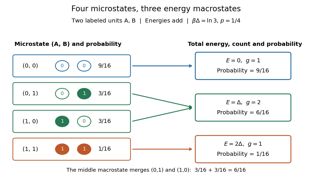
A macrostate groups microstates sharing prescribed coarse data. The grouping depends on what is retained: here retain only total energy. For the two distinguishable two-level systems, the macrostates $E=0,\Delta ,2\Delta$ have state degeneracies $1,2,1$. Although two units are not macroscopic in size, they make this loss of information visible: knowing $E=\Delta$ does not tell us which unit is excited.

At inverse temperature $\beta \Delta =\ln 3$, each unit's excited-state probability is $p=1/4$. Their independence gives microstate probabilities $9/16,3/16,3/16,1/16$ in the order above. Adding within each macrostate givesThe total expected value of energy is therefore $\Delta (6/16)+2\Delta (1/16)=\Delta /2$, matching two units each with expected value of energy $\Delta /4$. Equal state degeneracies would give the wrong answer: macrostate probabilities combine counting with the Boltzmann factor. At very high positive temperature, all four microstates become equally likely, but these three macrostate probabilities approach $1/4,1/2,1/4$.

A microstate is a complete microscopic specification within the chosen model. For two distinguishable, noninteracting two-level systems, label the units $A,B$ and their states $0,1$, with energies $0,\Delta$ and $\Delta >0$. The four microstates arewith total energies $0,\Delta ,\Delta ,2\Delta$. Distinguishability matters: $(0,1)$ and $(1,0)$ describe different assignments to the labeled units. Noninteraction matters too: their energies add without an extra coupling term.

For a classical particle model, a microstate can instead be a point in phase space, specifying every position and momentum. In the quantum canonical ensemble, the sum uses energy eigenstates; a general quantum state may also contain quantum coherence, which an energy label alone does not specify.

A degeneracy factor counts distinct microstates sharing the same specified energy or other grouped quantum labels. If an energy level $E_i$ has multiplicity $g_i$, its contribution to the canonical partition function is $g_i{e}^{-\beta E_i}$. The probability of occupying that entire level is consequently proportional to both its Boltzmann factor and its state degeneracy.

For a lower nondegenerate level at zero energy and an upper level at $\Delta$ with degeneracy factor $g$, the upper-level probability is $g{e}^{-\beta \Delta }/(1+g{e}^{-\beta \Delta })$. Equal level probabilities occur at $\Delta =k_{B}T\log g$, rather than necessarily at equal energies. This makes state counting a source of observable entropic shifts. The multiplicity must match what has already been counted explicitly; summing separately over spin states and then multiplying by the same spin multiplicity would double-count microstates.

A Standard Model generation contains left-handed quark and lepton doublets and right-handed up-quark, down-quark and charged-lepton singlets. A right-handed neutrino may be added as a gauge singlet.

The electroweak interaction is the $SU(2{)}_L\times U(1{)}_Y$ gauge theory that unifies the weak and electromagnetic interactions.

An instructive tension motivates the unification: the photon is massless, while the W boson and Z boson are massive; electromagnetic interaction and weak interaction also have different observed low-energy strengths and chiral couplings. A gauge theory can relate their interactions while the Higgs field gives different masses after electroweak symmetry breaking. The resulting theory predicts relationships between processes, not merely a common name for observed phenomena.

Its useful organizing principle is the combination of weak isospin and hypercharge. The surviving electromagnetic generator is $Q=T_3+Y$ in the convention used here. The photon and Z boson are different mixtures of neutral gauge fields, while the charged current uses the charged combinations. The electroweak doublet gauge-boson mass matrix explains why one neutral mixture stays massless. At low energies, a massive W boson propagator instead produces the approximate Fermi interaction, withHere $g$ is the $SU(2{)}_L$ gauge coupling and $v$ the Higgs doublet vacuum expectation value. The inverse squared mediator mass suppresses low-energy weak rates. Unification does not require setting $g$ equal to the electromagnetic coupling $e$: their relation is $e=g\sin {\theta }_W$.

A striking experimental consequence is a neutral current in addition to the familiar charged current. The Gargamelle experiment tests this extra channel through visible charged secondaries, with a background problem fundamentally different from directly identifying a Z boson. The muon-neutrino electron recoil spectrum shows how the same Weinberg angle enters another process quantitatively.

A nonlinear sigma model has fields valued in a curved target space such as a vacuum manifold $G/H$. Its leading action is quadratic in spacetime derivatives but nonlinear in any unconstrained coordinates used for the target.

In a local quantum field theory obeying special relativity, with a positive physical state space, a conserved continuous internal global symmetry in field theory and a selected Lorentz-invariant ground state, a broken generator requires a massless Goldstone boson. For $G\to H$, there are $\dim G-\dim H$ symmetry-required Goldstone bosons in this setting; additional accidental massless excitations are possible. Jeffrey Goldstone's institutional biography identifies his work with Abdus Salam and Steven Weinberg on the zero-mass theorem.^[ref]

The Goldstone directions in the scalar mass matrix give a short classical proof at a smooth minimum. The quantum argument uses a conserved current $j^{\mu }$ and a scalar local operator $O$ whose expectation changes under the broken generator. The Ward identity for the current–local operator correlation function then has a nonzero contact term. After a Fourier transform, its divergence remains nonzero as four-momentum tends to zero. Lorentz invariance forces the vector–scalar correlator to have the form $p^{\mu }F(p^2)$, so $F$ must have a pole at $p^2=0$. The spectral representation associates that pole with a physical zero-mass excitation. A properly regulated spatial integral of the conserved current implements the broken generator; a well-defined global charge acting on the broken ground state cannot simply be assumed.

The hypotheses explain the boundaries of the result. A discrete symmetry has no infinitesimal generator and need not give a Goldstone boson. A gauge redundancy does not supply the physical global generator assumed here. In nonrelativistic matter the type-B Goldstone boson shows why one cannot universally count one independent mode per broken generator. Long-wavelength fluctuations can also prevent an assumed broken state from existing, as in the Mermin-Wagner theorem.